
Danidutch
Danielefrancodetoledo
Recently Published


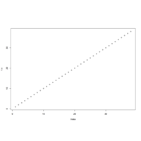
Plot
library(manipulate)
manipulate(plot(1:x), x= slider(1,100))
Peer graded Assigment R Markdown
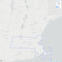
# Map the sites data using the leaflet package.
library(leaflet)
library(maps)
library(htmlwidgets) # To save the map as a web page.
# The data to map.
sites <- read.csv("http://college.holycross.edu/faculty/rlent/sites/sites.csv")
# State boundaries from the maps package. The fill option must be TRUE.
bounds <- map('state', c('Massachusetts', 'Vermont', 'New Hampshire'), fill=TRUE, plot=FALSE)
# A custom icon.
icons <- awesomeIcons(
icon = 'disc',
iconColor = 'black',
library = 'ion', # Options are 'glyphicon', 'fa', 'ion'.
markerColor = 'blue',
squareMarker = TRUE
)
# Create the Leaflet map widget and add some map layers.
# We use the pipe operator %>% to streamline the adding of
# layers to the leaflet object. The pipe operator comes from
# the magrittr package via the dplyr package.
map <- leaflet(data = sites) %>%
# setView(-72.14600, 43.82977, zoom = 8) %>%
addProviderTiles("CartoDB.Positron", group = "Map") %>%
addProviderTiles("Esri.WorldImagery", group = "Satellite") %>%
addProviderTiles("Esri.WorldShadedRelief", group = "Relief") %>%
# Marker data are from the sites data frame. We need the ~ symbols
# to indicate the columns of the data frame.
addMarkers(~lon_dd, ~lat_dd, label = ~locality, group = "Sites") %>%
# addAwesomeMarkers(~lon_dd, ~lat_dd, label = ~locality, group = "Sites", icon=icons) %>%
addPolygons(data=bounds, group="States", weight=2, fillOpacity = 0) %>%
addScaleBar(position = "bottomleft") %>%
addLayersControl(
baseGroups = c("Map", "Satellite", "Relief"),
overlayGroups = c("Sites", "States"),
options = layersControlOptions(collapsed = FALSE)
)
invisible(print(map))