
gill1109
Richard Gill
Recently Published

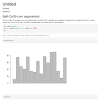
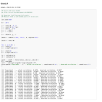
Simulation of Bell's LHV model; CHSH experiment
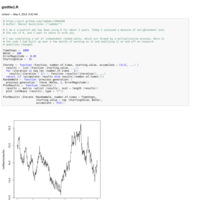
This script does the CHSH experiment 10,000 times under the assumption of local hidden variables, and more specifically, using Bell's own "by way of example" model
Hook Effect
The Hook effect. How immunoassay of the ELISA kind can sometimes report a concentration of almost zero, when actually the concentration is very large.
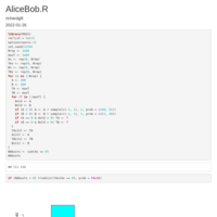
Lucy Letby - the spreadsheet
An important piece of evidence in the trial of Lucy Letby was a spreadsheet showing nurses' presence at a list of alledly suspicious incidents. This script reproduces the spreadsheet in a different format and places it next to a simulated spreadsheet where nurse x incident cells have been filled completely at random, but matching the observed total numbers for day shifts and night shifts (except for Lucy's shifts). This corresponds to a model in which incidents are thought to be suspicious merely because Lucy Letby is present.
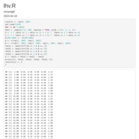
LHV-full
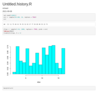
This is a simulation of a simple local hidden variables model for a standard Bell experiment (2 parties, 2 possible settings per party, 2 possible outcomes per party and setting). It results in correlations +0.5 for three setting pairs and -0.5 for the fourth. I simulate 100 times the experiment in which each setting paiir is used 25 times. The point is to notice that observed values of "S" vary widely around the mean value of 2; in half of the experiments we observe a violation of the CHSH inequality and in quite a few of them, rather a big violation.
Geurdes
Four times, 100 replications of a Bell experiment with 100 trials under each of the four setting pairs (thus 400 "particle pairs" per experiment). For discussion of a paper by Han Geurdes on https://www.qeios.com/read/V11ZO2 The underlying probability distribution of the data corresponds to the standard example local hidden variables model achieving S = 2 with all marginal expectations zero, three correlations of +0.5, one of -0.5
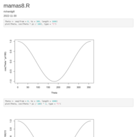
mamas 8
The graph of cos^2(theta) is a scaled and shifted version of a graph of cos(theta). Take careful notice of the numbers marked on the axes.
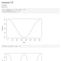
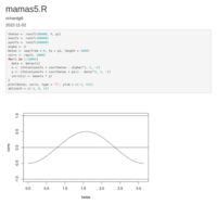
mamas 7
Yet another plot for Dean Mamas
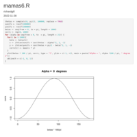
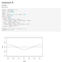
Mamas. 6
This time the photon pairs are with equal probabilities H, V and V, H. The correlation between the outcomes depends not only on the difference between the two settings but also on their relative position relative to H (zero) and V (ninety degrees).
Document
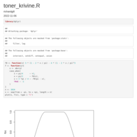
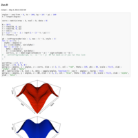
This is a simulation of the LHV defined by Ben Toner in his PhD thesis, in which he converts Krivine's derivation of the Grootendieck constant K_G(2) into a local hidden variable for a Bell experiment where Alice and Bob choose settings from the unit circle and the observed correlations are the -cos(alpha - beta) / sqrt 2.
Document
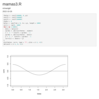
Dean Mamas, continued.
Document
Another version of Dean Mamas' model
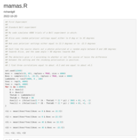
Document
Dean Mamas' model of a Bell experiment. The particles immediately become disentangled as they leave the source. The probabilities of detection are the absolute values of cosines of differences of polarization angles ....
Dean Mamas
A guy called Dean Mamas thinks that Bell was wrong. He published a one page paper in some not very high profile journal and is angry that nobody takes any notice of it. He believes in an establishment conspiracy. I hope he is able to learn "R" and I hope he is able to learn from experience.
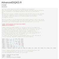
Advanced DIQKD
Continuation of OptimizedDIQKD. I now further sharpen the results by estimating the 8 parameters of the multinomial (No-Signalling) model by maximum likelihood, and also estimating the 7 parameters of the submodel obtained by restriction to Local Realism.
Statistical testing is probably improved by using the Wilks minus two log likelihood ratio test (compared to the chi-squared distribution with one degree of freedom), instead of a Wald test based on an estimated parameter and estimated asymptotic variance.
First we simply re-run the generalised least squares program in order to get initial estimates of the parameters under the unrestricted model, and we rerun a modification thereof to get initial estimates under the restriction that S = 2 (J = 0)
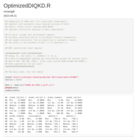
Optimized DIQKD
Comparison of CHSH and J for recent Bell experiments, together with optimally noise-reduced versions of both. Theory: https://arxiv.org/abs/2209.00702, "Optimal statistical analyses of Bell experiments". This experiment: Zhang, W., van Leent, T., Redeker, K. et al. A device-independent quantum key distribution system for distant users. Nature 607, 687–691 (2022). https://doi.org/10.1038/s41586-022-04891-y. Data obtained from Timm van Leent
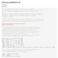
AdvancedWeihs
following on from "OptimisedWeihs" we go on to calculatte the Wilks likelihood ratio test, extra a probably more exact z-value from it, and from that a more realistic p-value using good old-fashioned Chebyshev. See https://arxiv.org/abs/2209.00702 for the theory.
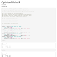
Optimised Weihs
Comparison of CHSH and J for Weihs classic Innsbruck experiment, together with optimally noise-reduced versions of both. Theory: see https://arxiv.org/abs/2209.00702, Optimal statistical analyses of Bell experiments. (Richard D. Gill) We show how both smaller and more reliable p-values can be computed in Bell-type experiments by using statistical deviations from no-signalling equalities to reduce statistical noise in the estimation of Bell's S or Eberhard's J.
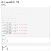
OptimisedDelft_2.R
Comparison of CHSH and J for the Delft experiment, together with optimally noise-reduced versions of both. Theory: Comparison of CHSH and J, together with optimally noise-reduced versions of both, see https://pub.math.leidenuniv.nl/ ~gillrd/Peking/Peking_4.pdf In short: assume four multinomial samples, estimate covariance matrix of estimated relative frequencies, use sample deviations from no-signalling to optimally reduce the noise in the estimate of Bell's S or Eberhard's J
Document
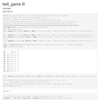
Bell games

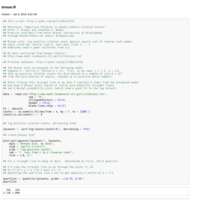
KillerNurse
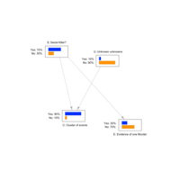
A Bayes net for a suspected serial killer nurse case. Allows for unknown factors to be able to cause a cluster of suspicious events involving a nurse. We may or may not also have strong evidence of ill-doing by our nurse for one patient. If we observe the cluster but no strong evidence our nurse harmed any particular patient, it's most likely the cluster was a coincidence. But if we observe both, things are serious (though still not clearcut)
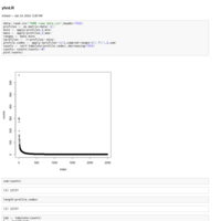
KillerNurse
Plot from KillerNurse2

KillerNurse
A Bayes net for a suspected serial killer nurse case. Allows for unknown factors to be able to cause a cluster of suspicious events involving a nurse. We may or may not also have strong evidence of ill-doing by our nurse for one patient. If we observe the cluster but no strong evidence our nurse harmed any particular patient, it's most likely the cluster was a coincidence. But if we observe both, things are serious (though still not clearcut)
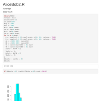
Alice and Bob in the New Yorker, continued
Alice and Bob problem
Alice and Bob in the New Yorker
Alice and Bob problem
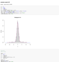
Document
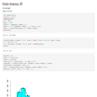
Fitting a probability density by smoothing a histogram. Square root transformation to stabilise the variance.
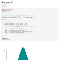
Illustration of Gill's Spreadsheet Theorem
Illustration of Gill's Theorem 1 in https://arxiv.org/abs/1207.5103 "Statistics, Causality, and Bell's Theorem), Statistical Science 2014, Vol. 29, No. 4, 512-528.
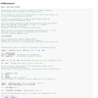
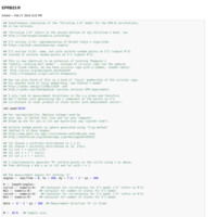
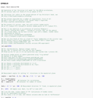
Simulations of EPR-B experiment
I simulate the results of a perfect EPR-B experiment using setting pairs with difference equal to 0, 1, ... 360 degrees; for each each angle pair, N = 1e02, 1e04, and 1e06.
Daniela Poggiali
Some important graphics concerning shifts and deaths in medium care wards A, B, C and D combined. Daniela Poggiali (like most nurses) works most hours when most deaths occur (or rather: are registered as having occurred): during the morning shift.

Daniela Poggiali
Did Daniela Poggiali kill patient Mrs Calderoni? Is she in fact the one of the greatest health-care serial killers in history? I show that statistical evidence that she killed more than 80 patients actually does not make it likely that she murdered one particular patient. The prior beats the likelihood ratio. A p-value of 1 in one thousand sounds impressive but doesn't match up to a prior of 1 in a million.
CoronaOrigins
A Bayes net investigating the source of the Corona pandemic
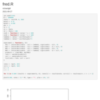
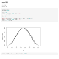
Fred
Fred Diether's latest simulation of an EPR-B experiment
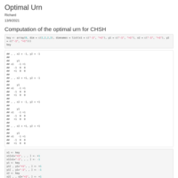
Optimal urn
Computation of the optimal urn for the CHSH urn model
CHSH urn model 2
A random urn used to build a simulation of a CHSH urn model; and an optimal urn too.
CHSH urn model
A random urn used to build a simulation of a CHSH urn model
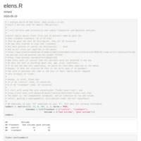
Elens
Dutch family doctor Rob Elens first had 25 patients whom he gave the then standard treatment; and 12 of 25 died. Then he gave the next 8 chloroquine, and they all 8 recovered. He was then ordered to stop that treatment. His next patient of course (no chloroquine) ... died. So his story was taken up by the media... now read on.
Raoult6
The most simple Bayesian model yet...
Raoult5
This is a Bayesian analysis of the Marseilles trial using JAGS and MCMC. This time I use a different Bayesian model which I think is more intuitive. Moreover, I add a simulated one new patient from each group and print their joint distribution. This time I have created a "slab and spike" prior distribution on the unit square. It's a 50-50 mixture of a uniform density on the unit square, and a uniform density on a strip about the main diagonal of width sqrt 2 times 0.1.
Raoult4
Marseilles trial, best analysis ever (though still without covariates to take account of *known* possible confounders)
Raoult3
I again run the Bayesian analysis of the Marseilles trial using MCMC. This time I use a different Bayesian model to the one standardly employed by JAGS. I again use rjags with a new model defined in the BUGS language, which I think is more intuitive.
Raoult2
Bayesian model of the Marseilles trial analysed by MCMC. This comes down to an analysis with MCMC using the BUGS model implemented in the application JAGS.
Raoult
Very simple analysis of the Raoult trial (new treatment in Nice versus standard treatment in Marseilles. Uses ITT principle. Fisher's exact test, Barnard's test, and the Bayesian pabtest from the application JASP.
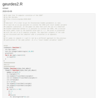
Geurdes2
R code from "A computer violation of the CHSH” by Han Geurdes, https://vixra.org/abs/1910.0423 Abstract: If a clear no-go for Einsteinian hidden parameters is real, it must be in no way possible to violate the CHSH with local hidden variable computer simulation. In the paper we show that with the use of a modified Glauber-Sudarshan method it is possible to violate the CHSH. The criterion value comes close to the quantum value and is > 2. The proof is presented with the use of an R computer program. The important snippets of the code are discussed and the complete code is presented in an appendix.
It seems to compute 1 + sqrt 2, but by a different approach to the previous publication of the same author. Is it a "local hidden variables" model?
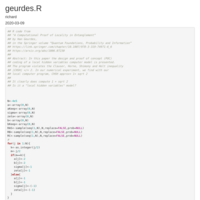
Geurdes
R code from "A Computational Proof of Locality in Entanglement”by Han Geurdes, in the Springer volume “Quantum Foundations, Probability and Information https://link.springer.com/chapter/10.1007/978-3-319-74971-6_6 https://arxiv.org/abs/1806.07230 Abstract: In this paper the design and proof of concept (POC) coding of a local hidden variables computer model is presented. The program violates the Clauser, Horne, Shimony and Holt inequality CHSH| </= 2. In our numerical experiment, we find with our local computer program, CHSH approx= 1+ sqrt 2.
It clearly does compute 1 + sqrt 2. Is it a "local hidden variables" model?
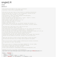
Spinning disk model of the singlet correlations
Here I test the spinning disk model of the singlet correlations, choosing parameters of the model at random. The simulation shows that it is not true that quantum correlations are necessarily *stronger* than classical correlations. A few of the simulated models have correlations stronger than those seen in the quantum negative cosine curve.
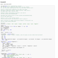
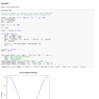
Testing Chantal’s simulations
This is a test of the java application being developed here:
https://github.com/chenopodium/Eberhard
AdvancedDelft
I now further sharpen the results by estimating the 8 parameters of the multinomial (No-Signalling) model by maximum likelihood, and also estimating the 7 parameters of the submodel obtained by restriction to Local Realism.
Statistical testing is probably improved by using the Wilks minus two log likelihood ratio test (compared to the chi-squared distribution with one degree of freedom), instead of a Wald test based on an estimated parameter and estimated asymptotic variance.
There are some surprising differences! Physicists should learn some textbook small-data statistical theory especially if their sample sizes are big!

AdvancedVienna
I now further sharpen the results by estimating the 8 parameters of the multinomial (No-Signalling) model by maximum likelihood, and also estimating the 7 parameters of the submodel obtained by restriction to Local Realism.
Statistical testing is probably improved by using the Wilks minus two log likelihood ratio test (compared to the chi-squared distribution with one degree of freedom), instead of a Wald test based on an estimated parameter and estimated asymptotic variance.
There are some surprising differences! Physicists should learn some textbook small-data statistical theory especially if their sample sizes are big!
AdvancedNIST
I now further sharpen the results by estimating the 8 parameters of the multinomial (No-Signalling) model by maximum likelihood, and also estimating the 7 parameters of the submodel obtained by restriction to Local Realism.
Statistical testing is probably improved by using the Wilks minus two log likelihood ratio test (compared to the chi-squared distribution with one degree of freedom), instead of a Wald test based on an estimated parameter and estimated asymptotic variance.
There are some surprising differences! Physicists should learn some textbook small-data statistical theory especially if their sample sizes are big!
AdvancedMunich
I now further sharpen the results by estimating the 8 parameters of the multinomial (No-Signalling) model by maximum likelihood, and also estimating the 7 parameters of the submodel obtained by restriction to Local Realism.
Statistical testing is probably improved by using the Wilks minus two log likelihood ratio test (compared to the chi-squared distribution with one degree of freedom), instead of a Wald test based on an estimated parameter and estimated asymptotic variance.
There are some surprising differences! Physicists should learn some textbook small-data statistical theory especially if their sample sizes are big!
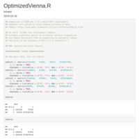
OptimizedVienna
Comparison of CHSH and J for the Vienna experiment, together with optimally noise-reduced versions of both. Theory: Comparison of CHSH and J for the NIST experiment, together with optimally noise-reduced versions of both.
Theory: https://pub.math.leidenuniv.nl/
~gillrd/Peking/Peking_4.pdf
In short: assume four multinomial samples, estimate covariance matrix of estimated relative frequencies, use sample deviations from no-signalling to optimally reduce the noise in the estimate of Bell's S or Eberhard's J
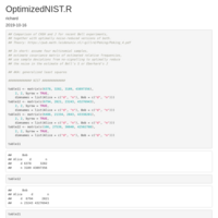
OptimizedNIST
Comparison of CHSH and J for the NIST experiment, together with optimally noise-reduced versions of both.
Theory: https://pub.math.leidenuniv.nl/
~gillrd/Peking/Peking_4.pdf
In short: assume four multinomial samples, estimate covariance matrix of estimated relative frequencies, use sample deviations from no-signalling to optimally reduce the noise in the estimate of Bell's S or Eberhard's J
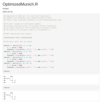
OptimizedMunich
Comparison of CHSH and J for the Munich experiment, together with optimally noise-reduced versions of both. Theory: Comparison of CHSH and J for the NIST experiment, together with optimally noise-reduced versions of both.
Theory: https://pub.math.leidenuniv.nl/
~gillrd/Peking/Peking_4.pdf
In short: assume four multinomial samples, estimate covariance matrix of estimated relative frequencies, use sample deviations from no-signalling to optimally reduce the noise in the estimate of Bell's S or Eberhard's J
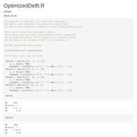
OptimizedDelft
Comparison of CHSH and J for the Delft experiment, together with optimally noise-reduced versions of both. Theory: Comparison of CHSH and J for the NIST experiment, together with optimally noise-reduced versions of both.
Theory: https://pub.math.leidenuniv.nl/
~gillrd/Peking/Peking_4.pdf
In short: assume four multinomial samples, estimate covariance matrix of estimated relative frequencies, use sample deviations from no-signalling to optimally reduce the noise in the estimate of Bell's S or Eberhard's J
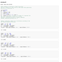
chili
Plots belonging to (2015) correction note of Brummert Lennings & Warburton (2011)
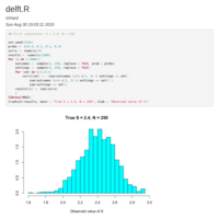
delft
The Delft experiment - three different scenarios
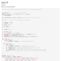
joy1
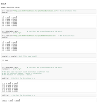
Counting the number of accepted particle pairs in Joy Christian's http://rpubs.com/jjc/84238
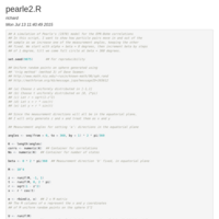
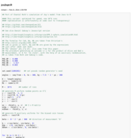
pearle2
A simulation of Pearle's (1970) model for the EPR-Bohm correlations. In this script, I want to show how particle pairs move in and out of the sample as we increase one of the measurement angles, keeping the other fixed. We start with alpha = beta = 0 degrees, then increment beta by steps of 1 degree, till we come full circle at beta = 360 degrees. The sample size is small (10^4) to make for a fast running script.
minkwe
I analyse the data generated by M. Fodje's simulation programs "epr-simple" and "epr-clocked" using appropriate modified Bell-CHSH type inequalities: the Larsson detection loophole adjusted CHSH, and the Larsson-Gill coincidence loophole adjusted CHSH. The experimental efficiencies turn out to be approximately eta = 81% and gamma = 55% respectively, and the observed value of CHSH is (of course) well within the adjusted bounds.
epr-clocked-full
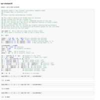
Michel Fodje's "epr-clocked" now with all bells and whistles, together with verification that the simulation results do not violated the Larsson-Gill corrected CHSH inequality (corrected for coincidence post-selection)
epr-clocked-core
Michel Fodje's "epr-clocked", core part of model, many different performance metrics. In particular, verification that the simulation results do not violate the Larsson-Gill (2004) corrected CHSH inequality - corrected for coincidence loophole post-selection.
Christian's latest attempt
Joy Christian's http://rpubs.com/jjc/84238; Two lines added in order to illustrate varying sample sizes. Nothing else changed. It would be interesting to also study the overlap between the different samples. I'm thinking about how to visualise that in a sensible way.
onion2
An attempt to save Christian's one page paper by applying Albert Jan's patch to the central bug.
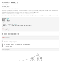
tree2
More fun with trees, in order to help visualising the junction tree algorithm
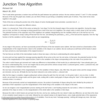
tree.Rmg
Draw a random tree with two nodes and the path between them marked by different colours. Part of attempt to explain the junction tree algorithm ...
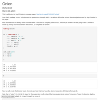
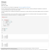
onion
Test of Joy Christian's "one page paper" model http://arxiv.org/pdf/1103.1879v1.pdf of the singlet correlations.
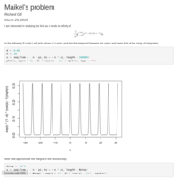
maikel
Investigation of convergence of an integral in Esty's proof of the asymptotic normality of the Good estimator.
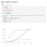
MLE_SMLE_script
Figure 1.7 of Groeneboom and Jongbloed (Bangkok data)
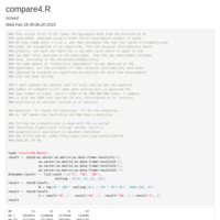
compare4
Comparison of various CH variants, and CHSH, for Giustina et al (fixed grid of coincidence windows, width = 50 time stamp units)
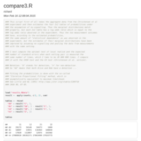
compare3
Compute optimal test of local realism for Christensen et al. data
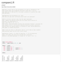
compare1
Comparison of statistical power of CHSH and CH in ideal experiment. Also, comparison of aggregate data from Christensen et al. paper and as recomputed by me
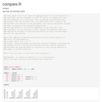
compare
Comparison of Clauser-Horne and CHSH on Christensen et al. data.
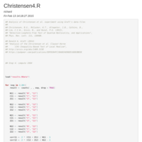
Christensen4
Analysis of Christensen experiment starting from Graft's data: step 4: CHSH
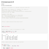
Christensen3
Analysis of Christensen et al. experiment from Graft's data, step 3: computation of B and B' (normalized Clauser-Horne) for all 20 data-sets
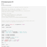
Christensen2
Analysis of Christensen et al. experiment from Graft data. Step 2. Reduction to set of coincidence counts, singles counts, and empty window counts, for all 20 data-sets
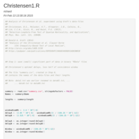
Christensen1
Analysis of Christensen et al. data from Graft's data. Step 1, reduction of the data to small binary files, one for each experiment.
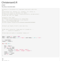
Christensen0
Analysis of Christensen et al. data using Graft's data sets. Step 0. Preparations.
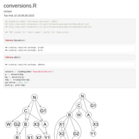
conversions
Yet more exercises with R graphical models programs
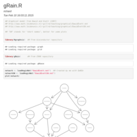
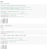
gRain
Some quick exercises with graphical models in R
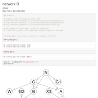
network
More advanced exercises with R and graphical models
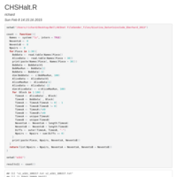
CHSHalt
Giustina et al again, fixed time-slots, this time of 980 ns instead of 1000 ns
CHSH
Analysis of Giustina et al. data using fixed 1000 nanosecond time-slots and coarse-graining: the two outcomes are: "one of more events in time-slot"; "no events in time-slot"
CH
Getting the statistics out of the raw data of the Giustina et al. experiment

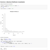
zipf
An illustration of the Zipf law and a new estimation method
spreadsheet
Generates a spreadsheet and random settings such that the Bell-CHSH inequality is resoundingly violated (and quantum mechanics prediction for the singlet state confirmed) at N = 800, http://arxiv.org/abs/1207.5103
JustinLee3
See my RPubs documents JustinLee, and JustinLee2. This is the same as JustinLee2, zooming in to see more clearly the difference between the two correlation curves ...

JustinLee2
See my RPubs document JustinLee. This is the same but with slightly different parameters. We get a bigger violation of CHSH but smaller efficiencies ...

JustinLee
A simulation of Justin Lee's (2014) precession model for the EPR-Bohm correlations http://vixra.org/abs/1408.0063 "Bell's Inequality Loophole: Precession"
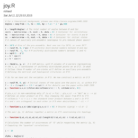
joy
Adaptation of Joy Christian's script http://rpubs.com/jjc/16415, now we just print out the four correlations for the four combinations of angles in a CHSH experiment.
An error is corrected in http://rpubs.com/gill1109/80119
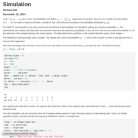
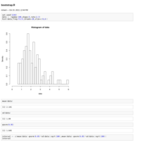
simulation
Simulation of diversity data from genomics, and a conjecture
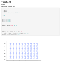
yoichi
Moving balls about
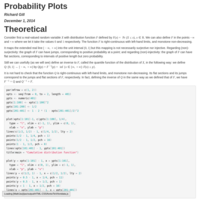
probplots
Notes on probability plots, quantile plots, QQ plots ... to be expanded with R illustrations
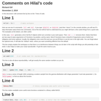
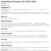
Uitleg
Uitleg over Hilal Moussa's code
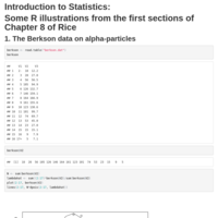
ist130903
Course "Introduction to Statistics", some R illustrations from Rice chapter 8
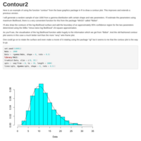
contour2
Here is an example of using the function “contour” from the base graphics package in R to draw a contour plot. This improves and extends a previous version.
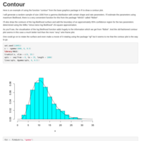
contour
Illustration of R base graphics function "contour"
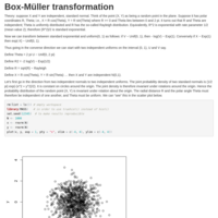
boxmueller
Visualisation of Box-Müller transformation

Opinion
Working document - are respiratory arrests rare in the Emergency Department of a hospital like Horton General (Banbury, UK)? (cf. case of Ben Geen).
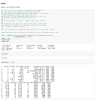
esb.R
Alternative vs. official ESB ranking of Dutch economists according to Abbring et al.
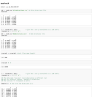
testFred.R
Test of Fred Diether III's submission to the Christian experiment data challenge
test.R
My test program applied to Christian's latest submission to my challenge
epr-clocked.R
Michel Fodje's "epr-clocked" coincidence loophole model, stripped down to essential core https://github.com/minkwe/epr-clocked
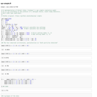
epr-simple.R
Michel Fodje's epr-simple simulation of the singlet correlations, run under the protocol of a delayed choice, event-ready-detectors, Bell-CHSH type experiment
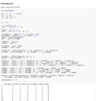
Coincidence.R
Test

Coincidence.R
Simulation of the Larsson-Gill coincidence loophole model. Parameters chosen to exactly reproduce CHSH = 2 sqrt 2. Sample size N = 10^4. This sample coincidentally just violates the Larsson-Gill population bound, though not significantly, if we take standard errors into account and use a reasonable significance level.
gistfile1.R
"lambder" 's "Zen of R" https://gist.github.com/lambder/2066588
Zen.R
Zen's surface plot of Joy's simulation
christian.R
Test of Christian's claim to 10 000 Euro. Result = fail. Please try again, Joy.
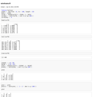
bet2.R
Version 2 of the code for deciding the bet between Christian and Gill, concerning the results of Christian's exploding ball experiment. This version: each correlation is based on a different sample, chosen at random, completely disjoint.
wireframe.R
The quantum correlation surface and the points on it of a CHSH-style experiment. Angles in degrees, from 0 to 180.
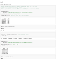
bet.R
Draft protocol of final stage of bet with Joy Christian. The two data sets will be replaced by data sets generated in his experiment.
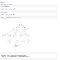
gRain.R
Dawid and Evett network
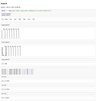
fred3.R
Illustration of Theorem 1 of my "Statistics, Causality and Bell's Theorem" (the spreadsheet theorem), http://arxiv.org/abs/1207.5103
QRC.R
The quantum Randi challenge (Vongehr, 2012, 2013, ...) http://arxiv.org/abs/1207.5294
pearle.R
Simulation of the Pearle (1970) local hidden variables model
EPRB2.R
Minkwe's implementation of Christian's model, 2-d, R implementation by R D Gill
zen.R
Zen's modification of Joy's Experiment, adapted from Richard Gill's code, with constant shifts
joychristian.R
Joy's Experiment, adapted from Richard Gill's code, with constant shifts
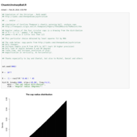
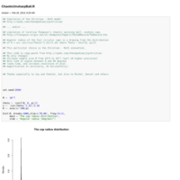
ChaoticUnsharpBall1.R
Gill - Thompson model. Chaotic rotating ball model with circular caps with radius R = ( 1 + U^gamma) * 45 degrees, where gamma = 0.46 is a bit smaller than 1/2
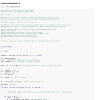
ChaoticUnsharpBall3.R
Computational proof that we can achieve the cosine exactly in the Joy Christian - Michel Fodje - Chantal Roth / Caroline Thompson - Richard Gill simulation model ... a convex combination of the blue curves will give us the black curve.
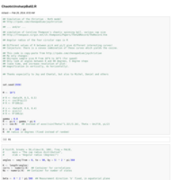
ChaoticUnsharpBall2.R
Script to investigate different radii distributions for the chaotic ball model / Christian-Roth model
ChaoticUnsharpBall.R
New name, but just a higher resolution performance of the Christian-Roth model http://rpubs.com/chenopodium/joychristian
EPRB2minkwe.R
Michel Fodje's model: theta_0 sampled from the discrete uniform on angles at steps of 7.5 degree between 0 and 90 degrees. To be precise: "0" included, "90" excluded in this code.
jcs2opt.R
Port of Chantal Roth's simulation of Joy's model from Java to R
This variant: optimised for speed, now 10^6 runs (optimisation is, of course, unfortunately at some cost to transparency!)
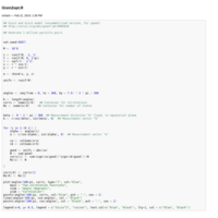
Gisin2opt.R
Gisin and Gisin model (unsymmetrized version, for speed)
http://arxiv.org/abs/quant-ph/9905018
jcs2.R
Port of Chantal Roth's simulation of Joy's model from Java to R. This variant: just one angle pair (alpha = beta = 0), but now 10^6 runs. The observed correlation is 0.98, not 1.
jcs.R
Port of Chantal Roth's simulation of Joy's model to R
https://github.com/chenopodium/JCS
https://github.com/chenopodium/JCS2
http://libertesphilosophica.info/eprsim/EPR_3-sphere_simulation5M.html
http://libertesphilosophica.info/eprsim/eprsim.txt
EPRB3opt.R
Optimized simulation of Joy Christian's S^2 (R^3) model.
EPRB23big.R
This is essentially the same script as my recent EPRB23.R. Comparison of two versions of Christian's/Minkwe's/Thompson's LHV models: S^1 (R^2) and S^2 (R^3). I only look at one angle but take the sample size equal to 100 million. 100 times larger than the previous, hence 10 times smaller standard error.
Gisin2.R
Gisin and Gisin EPR-B local hidden variables model:
http://arxiv.org/abs/quant-ph/9905018
Generate 1 million particle pairs.
Measure them in 20 random pairs of directions.
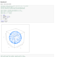
S2uniform.R
Sampling and plotting uniform random points on the uniform sphere
Chantal2.R
This is Chantal Roth's adaptation of my code of her model.
Additional features: try different "fudge factors"; compute CHSH.
Based on RDG's understanding of Chantal's java code at
https://github.com/chenopodium/EPR
This is still a "beta testing" version. Main missing feature: any explanation of what is going on!
EPRB23.R
Comparison of Michel Fodje's model 2D and 3D (S^1 and S^2) = Joy Christian's model = Caroline Thompson's model: "the chaotic spinning ball" (or disk) with random disk sphere cap radii.
chantal.R
Chantal Roth's local hidden variables model
EPRB3.R
Minkwe's implementation of Christian's model, 3-D, writen in R by R D Gill
yhrd.R
Y-str raw profiles plot
breuer.R
This is another try at modelling citation data according to Peter Breuer's model. This time I take the plot seriously and take the fitted straight line literally as a probability model. I show that data simulated according to this model is approximately log normally distributed
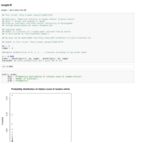
insight.R
Simulation of a citation count model - ideas due to Peter Breuer
solution week 2.html
Advanced Statistical Computing course, assignment for week 2

myknit.html
My first knitr attempt