
alobo
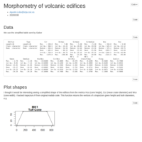
Agustin Lobo
Recently Published

Results of methods "bary" and "nnls" differ
While both unmixR::abundances() methods "bary" and "nnls" produce very similar results with the demo_data in the README.md example, the results strongly differ with a multi-spectral image.

Calculate and Display dissimilarity between 2 sets of Reflectance spectra
Comparing dissimilarity values to visual inspection of couples of most similar (NN) spectra
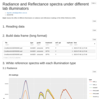
Test of lab illuminators (Std Reference)
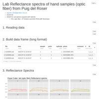
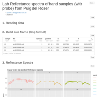
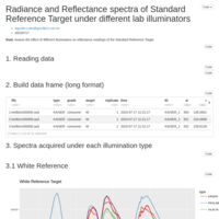
Reflectance spectra of the Standard Reference target under different lab illuminators
Test of lab illuminators
Radiance and Reflectance spectra under different lab illuminators
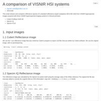
A comparison of VISNIR HSI systems
This script extracts and compares reflectance spectra of a standard reflectance target (Labsphere WCS-MC-020) from VISNIR hyperspectral images acquired with three VISNIR hyperespectral imaging systems in HSILab premises:
* Cubert Firefleye S185 SE
* Specim IQ
* Specim FX10

Specim IQ test of grey standards
Reflectance spectra of 2 grey standards from a VISNIR hyperspectral image acquired with a Specim IQ system in HSILab premises on 20221109:
* Specim IQ white reference card.
* Labsphere 50% reflectance standard
* Cubert grey reflectance standard
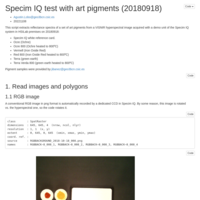
Specim IQ test with art pigments
Art pigments (control and heated to 800ºC) as imaged by hyperspectral camera Specim IQ
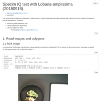
Specim IQ test with Lobaria amplissima (20180918)
Reflectance spectra (400 - 100 nm) of hydrated and dry samples of Lobaria amplissima extracted from a hyperspectral image (Specim IQ)
EndMembersRodalquilar2
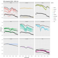
Comparison of EMs to spectral libraries (UGS+Ecostress) (2000-2460 nm)
Color: spectral libraries
Black: TFM
Grey: Bedini (height is approx.)
EndMembersRodalquilar
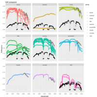
Comparison of EMs to spectral libraries (UGS+Ecostress)
Color: spectral libraries
Black: TFM
Grey: Bedini (height is approx.)

IQ_20180918_DIPV23
Specim IQ test 20180918_DIPV23

Options to calculate Reflectance
This script compares 4 options to calculate reflectance from radiance images acquired by hyperspectral scanning systems, in particular, Specim FX17 and FX10 mounted on desktop-size Lumo Scanner stands
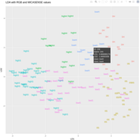
LDAall_RGBMICAv2b
LDA severuty all classes by segments P8
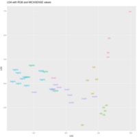
LDAall_RGBMICA
LDA severity by plots with M in P8

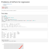
Problems witth lmPerm::lmp() for regression
Some problems with lmp described

spintutorial
Simple Markdown syntax for formatting your R scripts into WEB pages using knitr::spin()
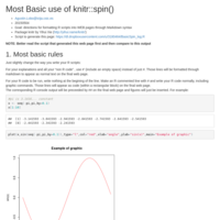
BasicSpin_log
Most Basic use of knitr::spin()
Val2013_V1V2comp_log
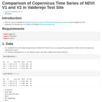
Comparisson of Copernicus Time Series of NDVI V1 and V2 in Valderejo Test Site (Val2013_V1V2comp_log.R)
alobokola2_log
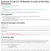
Exercise R Lab 2.1: Pollutants in soils of the Kola Peninsula
alobodaylength_log
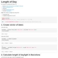
Length of Day
An example of computing with dates in R
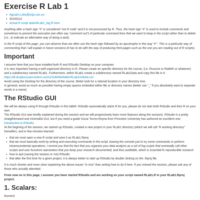
R Lab1
talleR ICTJA RLab1
test_log
to be removed
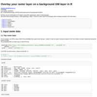
Overlay your raster layer on a background GM layer in R
GM tiles can be downloaded as R objects using either ggmap:get_map() or dismo:gmap().
We prefer dismo:gmap() because, unlike ggmap:get_map(), it returns a raster layer from package raster including complete CRS information
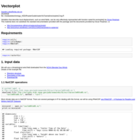
Vectorplot
Variables that describe local displacement, such as wind fields, can be very effectively represented with function rasterVis:vectorplot() by Oscar Perpinan.
We will use a climatological wind field dowloaded from the NOAA Blended Sea Winds
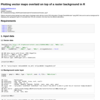
Plotting vector maps overlaid on top of a raster background in R
Objects returned by dismo:gmap() are raster layers of package *raster* with the correct CRS information ("Google PseudoMercator" epsg:3857) that can be used as background for displaying other geographic layers in R provided their CRS are consistent. We show here the different alternatives.
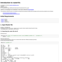
Introduction to rasterVis
rasterVis is an R package for the visualization of raster layers authored by Oscar Perpinan (http://oscarperpinan.github.io/)
This introductory material that does not substitute the standard documentation provided with the package and the documents provided by Oscar Perpinan:
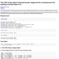
Finding out the CRS of the object returned by get_map()
The CRS of objects returned by get_map() is not documented. Here we use an empirical approach to confirm that, as it is usual in tools interacting with GM, the map is in so called "Google PseudoMercator" while coordinates are provided in "Longitude, Latitude" (datum WGS84 in both cases) and show how to produce correct plots of overlaid maps