
scblanco
Silvia Blanco
Recently Published

Generative AI: Knowledge is Power. Achieve in 1 day what others can't achieve in 6 months. Advanced Multi AI Agents: Use cases with Retrieval Augmented Generation (RAG)
Who said that knowledge is power? Of course, Silicon Valley, declaring that AI is the new electricity that transforms and improves all areas in human life. As a company, if you want nowadays your business to survive or - even better - thrive and be profitable, you need a strong competitive advantage and AI is the key. Just read on and prepare for a "wow" moment.
Renown global AI pioneer Andrew Ng, Professor at Stanford University (California), founder of DeepLearning.AI, co-founder of Coursera, founding lead of Google Brain, and former Chief Scientist at Baidu once told us during his courses that if you have the right know-how, you can achieve in 1 day what others can't achieve in 6 months – it's that simple. Hence my saying that work experience is no guarantee for competence or performance: in order to produce high quality, top performance work you need to possess know-how – and not just any, but the right one.
Thanks to cutting-edge AI technology launched this year, I've just been working on several practical use cases, including autonomous AI agents teams that produce a) Automated project planning breaking down projects, estimating time, and allocating resources. b) A progress report generator that interacts with project management tools. c) A sales pipeline that gets and enriches lead information, scores them, and drafts personalized emails for qualified leads. d) A customer support analysis pipeline that creates issue reports, visualizations, and makes suggestions for improvements. e) A content creation team that researches online, generates content, refines it, and creates social media posts.
This technology is not just amazing, but also extremely cost-effective: yes, that's right, absolutely awesome!
Take a tour on my other website for more info sblanco.netlify.app

AI Update / New Skills: New website for Generative AI - Multi-Agentic AI Skills
Have a look at my newly created website with a Gen-AI application that will help you caption your image. Enjoy!
https://huggingface.co/scblanco
Just finished a course on Multi-Agentic AI or multi-agent AI systems / workflows. It's a cutting-edge framework for orchestrating role-playing, autonomous AI agents that collaborate as a team to solve business problems. Example: Imagine you are the CEO of a start-up company with a tight budget, so you want AI to provide you with a 'virtual team' of highly skilled individuals. You can even expect a manager that supervises that team, delegates tasks, and coordinates them, all done autonomously. This technology will blow your mind, I promise - Silicon Valley doesn't sleep! Visit my other website for more info and a video link directly featuring the pioneer. https://sblanco.netlify.app/

AI update: Currently acquiring know-how directly from Silicon Valley's elite Stanford University and from Google: Deep Learning (neural networks) with TensorFlow
Silicon Valley (California, USA) is a global hub for technological innovation - where the future is being built - and home to industry titans like Google.
According to the QS World University Rankings 2025 of top global universities, Massachusetts Institute of Technology (MIT) is the absolute leader as number 1, followed closely by Harvard University (#4), and Stanford University (#6). Switzerland's ETH Zürich ranks currently #7. So, where are Neural networks being deployed? In our phones: to recommend content; In banks: to manage investments; In hospitals: to help doctors diagnose disease symptoms or interpret images and detect tumors; In insurance agencies: to evaluate risk and underwrite documents; In cars: to help avoid accidents. Up until now, my work in Artificial Intelligence (AI) was mainly focused on Discriminative AI: machine learning algorithms and other techniques applied for quantitative or qualitative statistical data analysis. As you may know, machine learning (ML) is a subset of AI, and deep learning is a subset of ML and uses neural networks to solve complex tasks. Neural networks can be used for complex, high dimensional classification tasks and I've posted one use case concerning smartphone preference months ago on this website. Other domains where Neural Networks are applied comprise computer vision, natural language processing, time series forecasting, speech recognition, etc. Some sophisticated applications in the area of natural language processing (NLP) consist of generative pre-trained transformers (GPTs) and the performance in this field improved considerably these last years. Today, everybody knows chatGPT, which is one area where these algorithms excel: (probability) models for generating new data. This type of AI is called Generative AI, and its capabilities are huge. As other tools are needed to dive deep into this area, I'm not posting on this website for now. You can find some more information on my other website: My web portfolio as business and AI strategist (sblanco.netlify.app) . See you soon!
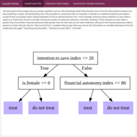
Prescriptive Analytics: Applied Econometrics - Causal Inference: Generalized random forests for policy evaluation. Case study: Evaluating the benefits of a financial education program in high schools in Brazil
The goal of every business is to optimize resource allocation and maximize results: Where should you focus your efforts to obtain a specific result? Who should you target so that customers do not churn and how should you prioritize them? Different business questions require different statistical models, and prediction (churn vs. not churn) is not the same as effect estimation or causality (identify the cause of churn so that you can prevent it from happening). For instance, being able to predict who is going to quit is not the same as determining who should your salespeople call so that they do not churn. In other words, who is more likely to be influenced by your action? A predictive model does not give you a set of rules to follow in order to attain maximum effect, because for that you need a prescriptive model. A logistic regression or other machine learning model can predict who is going to churn, but that is not the same statistical model you need if you wanted to identify those for whom you should intervene so that they do not churn and maximize your results. For that you need a causal model or a prescriptive analysis, not a predictive model. A causal forest is a nonparametric method for treatment effect estimation and predicts conditional average treatment effects (CATE). It offers the possibility to quickly identify important treatment modifiers in an experiment (or in an observational study), especially when you have a lot of them, in order to target the right people, cause the desired effect, and prioritize your actions. In the social sciences, for example in a marketing experiment, a causal forest performs much better than a traditional regression analysis or an ensemble method like classification and regression trees or random forests, and can be used for targeted advertising, uplift modeling, churn prevention, etc. In medicine, it aids at identifying target populations in preventive medicine. In this example, the benefits of a financial education program implemented in Brazil was evaluated. The experiment was randomized at the high school level and the dataset contains student-level data from around 17 000 students.
Source: Drexel University, LeBow College of Business / Stanford University, Graduate School of Business

Bayesian Inference – Hypothesis Testing. Advanced A/B testing in Marketing using Bayesian Decision Theory: Profit maximization with Test & Roll algorithm. Case study: Estimating the Returns to Advertising / Campaign ROI evaluation.
In 2015, Lewis and Rao wrote a paper named “The Unfavorable Economics of Measuring the Returns to Advertising” tackling the problem that major U.S. retailers face: Most of them reach millions of customers and collectively represent $2.8 million in digital advertising expenditure, but measuring the returns to advertising is difficult. Test & Roll A/B testing is a statistical technique in experimental design based in Bayesian decision theory and its goal is to maximize combined profit for both the test and the rollout phases. In the test phase you send out for example two versions of emails (in statistical jargon, the treatments), and in the roll phase you choose one version to deploy. Test & Roll finds the profit maximizing sample size for each phase using a Bayesian hierarchical model fit to past experiments data, run the Markov Chain Monte Carlo algorithm, and informs you the highest posterior probabilities of the parameters of interest; you then select the best option. In business terminology, this procedure allows to achieve maximum ROI (return on investment) with both the minimum sample size and the maximum profit possible, while yielding the lowest possible error rates. In contrast to the traditional hypothesis testing framework, sample sizes suggested by T&R are typically much smaller, which makes this approach more feasible as populations are limited and hypothesis tests don’t recognize this. Also, when a hypothesis test is statistically insignificant, it doesn’t tell you what to do, while Test & Roll shows exactly what alternative to choose and how much profit you would get. Finally, T&R works well when the response takes a long time to measure (long purchase cycles) and when iterative allocation would be time-consuming (email, catalog and direct mail).
Source: The University of Pennsylvania, The Wharton School, Wharton Customer Analytics Initiative
Inferential Statistics – Hypothesis Testing: Basic A/B testing in Marketing. Case study: Wine retailer emailing campaign experiment
A/B testing is a statistical technique in experimental design used to test a hypothesis and make data-driven decisions. It tests differences between two groups (for instance, control vs. treatment group) and is ideal for optimizing marketing campaigns, testing competing websites, assess reaction to advertisements, and so forth. In order to draw sound conclusions, A/B testing should be applied in conjunction with power analysis which is yet another statistical method used to determine the optimal sample size for yielding a significant effect with a high probability of occurrence (usually 80%) and minimum financial investment. Now, for the experiment to reach valid conclusions the experimental units should be randomized correctly. There are statistical methods to do this such as simple random sampling or other more sophisticated sampling methods to achieve this. In this example from a wine retailer, an experiment was conducted to answer the business question, "Which email version yields more sales?". An emailing campaign was carried out by randomly assigning customers to email versions A and B. A very basic A/B design experiment measures the 30-day purchase amount. Assumptions to identify the right A/B test are checked, then the appropriate test conducted, as well as a power analysis and a sample size calculation.
Source: The University of Pennsylvania, The Wharton School, Wharton Customer Analytics Initiative
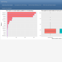
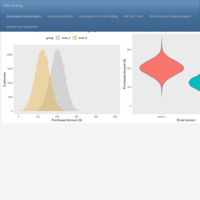
Inferential Statistics – Hypothesis Testing: A/B testing. Case study: Time spent on social media during COVID in India.
A/B testing is a statistical technique in experimental design used to test a hypothesis and make data-driven decisions. It is applied to test differences between two groups (control vs. treatment group) and is ideal for optimizing marketing campaigns, testing competing websites, assess audience reaction to advertisements, and the like. As with all experiments in a statistical design setting, A/B testing should be applied in conjunction with power analysis. Power analysis is yet another statistical method used to determine the optimal size of a sample that would yield a significant effect with a high probability of occurrence (usually 80%), so that you can derive sound conclusions that are based on an efficient use of the resources at hand (i.e. conduct the test with minimum financial investment). Under the umbrella of A/B testing and depending on the type of data you have, you can find: 1. Parametric tests: Independent samples t-test, paired (or dependent) samples t-test; 2. Nonparametric tests: Chi-Square test of independence, Mann-Whitney U test, Wilcoxon signed ranked test, and Fisher's Exact test. As a sidenote, A/B testing should only be applied to make comparisons between two groups (i.e. one factor variable restricted to two levels); the moment your experiment has more than two groups to compare (i.e. one or more than one factor variable with more than two levels), then an ANOVA (Analysis of Variance) is the right statistical tool for your analysis. Source: DataCamp
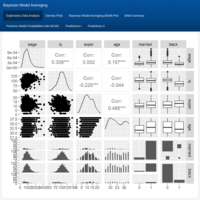
Bayesian Multiple Regression in Econometrics: Model selection using Markov Chain Monte Carlo (MCMC) algorithm. Case study: Finding the optimal model for predicting earnings.
In the field of labor economics, the study of income and wages provides insight ranging from gender discrimination to the benefits of higher education. But, what if you have 10,000 predictor variables? Often, several models are equally plausible and choosing only one ignores the inherent uncertainty involved in picking the variables to include in the model. A way to get around this problem is to implement Bayesian model averaging (BMA), in which multiple models are averaged to obtain posterior distributions. This cross-sectional wage dataset is a random sample of 935 respondents throughout the United States and has only 15 predictor variables; yet, that means there will be 32'768 potential predictive models (= 2^15 covariates). The more parameters there are in a model, the greater the in-sample goodness of fit (R-squared); however, this can lead to overfitting as additional terms may increase prediction error. Markov Chain Monte Carlo (MCMC) algorithm is useful when there are so many covariates that not all models can be enumerated. Instead of using stepwise selection to add or drop variables to improve a model like in OLS regression, MCMC finds the models with the highest posterior probability and provides unbiased estimates. In this simple example, MCMC is used in the context of Bayesian Model Averaging to sample models according to their posterior model probabilities, get model coefficients, and make predictions.
Source: Duke University, Department of Statistical Science
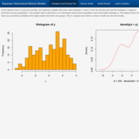
Bayesian statistics for hierarchical mixture modeling. Case study: Predicting population membership.
Histograms and density plots of data often reveal that they do not follow any standard probability distribution. Sometimes explanatory variables (or covariates) account for the different values. However, if only the data values themselves are available and no covariates, you might have to fit a non-standard distribution to the data. One way to do this is by mixing standard distributions, like two distributions governing two distinct populations in the data. Mixture distributions are just a weighted combination of probability distributions, such as one exponential and the other a normal distribution, or two normal distributions, and so on. In Bayesian statistics, one way to simulate from a mixture distribution is with a hierarchical model. In this example, the values observed belong to a group (i.e. population) that is unknown. Because these group variables are unobserved, they are called latent variables and can be treated as parameters in a hierarchical model and used to perform Bayesian inference.
Source: University of California, Santa Cruz - Department of Applied Mathematics and Statistics
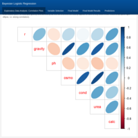
Bayesian Logistic Regression Modeling. Case study: Predicting the formation of calcium oxalate crystals in urine.
Urine specimens were analyzed in an effort to determine if certain physical characteristics of the urine might be related to the formation of calcium oxalate crystals. Variables in this dataset include: The specific gravity, pH reading, osmolarity, conductivity, urea concentration, and calcium concentration of the urine. Several of these variables show strong collinearity. Multicollinearity in linear regression models will compete for the ability to predict the response variable, thus leading to unstable estimates. If prediction of the response is the end goal of the analysis this is not a problem; but, as the goal of this analysis is to determine which variables are related to the presence of calcium oxalate crystals, collinearity of the predictors should be avoided and for that you need to conduct variable selection. One way to do that is to fit several sets of variables and see which model has the best Deviance Information Criterion (DIC) value. Another way to do it is to use a linear model where the priors for the linear coefficients favor values near 0, hence indicating a weak relationship. In this case, the prior to use is a double exponential or Laplace prior for the individual predictor variables. So the burden of establishing an association between variables lies with the data because if there is not a strong signal, then you can assume that it does not exist as the prior favors that scenario.
Source: University of California, Santa Cruz - Department of Applied Mathematics and Statistics
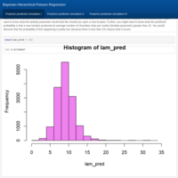
Bayesian statistics for hierarchical Poisson regression modeling II. Case study: Predicting chocolate chips in cookies produced at 5 different locations.
The model developed in part I is now used to get Monte Carlo estimates to make predictions. For example, from the posterior distributions obtained earlier, you can now simulate posterior predictive distributions to calculate the probability of some parameter of interest at a given existing location or even to get the mean number of chocolate chips per cookie for a new location that you might consider opening next.
Source: University of California, Santa Cruz - Department of Applied Mathematics and Statistics
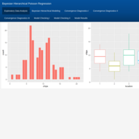
Bayesian statistics for hierarchical Poisson regression modeling I. Case study: Predicting chocolate chips in cookies produced at 5 different locations.
Hierarchical models extend basic statistical models to account for correlated observations. Bayesian statistics uses Markov Chain Monte Carlo to draw samples from a posterior (predictive) probability distribution, enabling you to simulate data taking into account uncertainty and allowing you to make more precise predictions. What makes Monte Carlo estimation powerful is the use of Gibbs sampling to update multiple parameters at the same time, simulate hypothetical draws from a probability distribution, and calculate parameters such as the mean or the variance, or the probability of some event, or quantiles of the distribution. In this example, a common statistical model for count data (Poisson regression) will be used for counting chocolate chips in cookies produced at 5 different locations. If all locations use the same recipe when they make their chocolate chip cookies, you would expect a cookie from one location to be more similar to another cookie from the same location/batch rather than to a cookie from another locations' batch. This means that when there's a natural grouping to the cookies (i.e. you have correlated data), you can no longer assume that all the observations are independent (which is a basic requirement of Poisson models). In such a case, you need a hierarchical model because observations are no longer independent. Should you fit five separate Poisson models (one for each location/batch of cookies), you would be ignoring data from other locations thus missing out on important information about the whole picture. Instead, hierarchical models share information, or borrow strength, from all the data and allow for more precise conclusions. A Bayesian hierarchical model will be specified, fitted, and assessed for convergence of the Markov chains and for overall model fit.
Source: University of California, Santa Cruz - Department of Applied Mathematics and Statistics

Bayesian Inference. Case study: Advertising campaign
Thanks to Bayesian inference, the British mathematician Alan Turing cracked the German Enigma code and helped secure the allied victory in World War II. He was able to decipher a set of encrypted German messages, searching the near-infinite number of potential translations as the code changed daily via different rotor settings on the complex Enigma encryption machine. Bayesian inference uses probability theory to draw conclusions about your data or the underlying parameters affecting it. Probability distributions represent uncertainty, and the role of Bayesian inference is to update these probability distributions (priors) to reflect what you learn from data in order to obtain a "posterior probability distribution" (i.e. conditioned probability). Bayesian inference requires data, a generative (statistical) model with priors, and a computational method. The key advantage of Bayesian inference is that it is highly flexible, allowing you to include information sources in addition to the observed data, such as background information, expert opinion or just common knowledge that you have and would like to add to the model. Hence your analysis results in a probability that is "conditioned" on some given assumption and this makes it is easier to use a Bayesian model to make an informed business decision. In this example, you run a website and want to get more visitors, so you are considering paying for an ad to be shown on a popular social media site that claims that their ads get clicked on 10% of the time. How can you be certain whether the investment is worth it? Moreover, you hear that most ads get clicked on 5% of the time, but for some ads it is as low as 2% and for others as high as 8%. How many more site visits is this campaign really going to generate? And what would happen if instead of clicks per ad you pay a banner per day? Bayesian inference allows you to answer all these questions.
Source: datacamp

Predictive Analytics / Machine Learning. Nonlinear Classifiers I: Decision Trees & Random Forests. Case Study: Smartphone Preference
Sophisticated classification methods for data analytics are required to handle large data sets with many features. Decision trees use heuristic processes (in this case, recursive partitioning) to determine the best order and cutoffs to use in making decisions and classify elements to divide and predict group memberships, allowing to incorporate complex interactions between variables. This is especially powerful when the structure of the classes are dependent or nested, or somehow hierarchical, when you have multiple categories, and when many of your observables are binary states (yes/no). A Random Forest is an 'ensemble' method: It combines the results of many small classifiers (i.e. in this case, trees) to make a better one. For large complex classifications, they can give probabilistic and importance weightings to each variable. In this example, a decision tree and a random forest were applied to analyze which personality factors can predict whether users report using an iPhone or an Android device. Key findings indicate that in comparison to Android users, iPhone owners were more likely to be female, younger, and increasingly concerned about their smartphone being viewed as a status object. Main differences in personality were also observed with iPhone users displaying lower levels of Honesty–Humility and higher levels of emotionality.
Source: Michigan Technological University – Applied Cognitive Science and Human Factors Program

Predictive Analytics / Machine Learning. Nonlinear Classifiers II: Artificial Neural Networks (ANNs). Case Study: Smartphone Preference
When complexity scales large, sophisticated classification methods for data analytics are required to handle large data sets with many features. The main advantage of ANNs are the use of hidden layers, which control how complex the classification structure is and solve the XOR problem: when a class is associated with an exclusive or logic. A simple two-layer neural network can be considered similar to a multinomial regression or logistic regression model, where inputs include a set of features, and output nodes are classifications that are learned. ANNs estimate weights, which are done with heuristic error-propagation approaches rather than maximum likelihood estimation (MLE) or least squares. While this is inefficient for two-layer problems, the heuristic approach will pay off for more complex problems with several hidden layers. In this example, a simple two-layer neural network was applied to analyze which personality factors can predict whether users report using an iPhone or an Android device.
Source: Michigan Technological University – Applied Cognitive Science and Human Factors Program
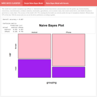
Predictive Analytics / Machine Learning: Naïve-Bayes Classifier. Case Study: Smartphone Preference
This classifier uses Bayes rule to combine information about a set of predictors. Naïve-Bayes (NB) combines all features equally – for each feature computing the likelihood of each option, and combining those one at a time, which also permits combining prior probability (base rate). One benefit of Bayes Factor is that is useful for data that are often likely to be missing. Another advantage is that it allows to estimate each feature empirically with the use of kernels. In this example, the NB method is applied to analyze which personality factors can predict whether users report using an iPhone or an Android device.
Source: Michigan Technological University – Applied Cognitive Science and Human Factors Program

Power Analysis / Sample Size Calculation I.
Power analysis is the statistical procedure used to determine if a test contains enough power to draw a reasonable conclusion. Power is the probability of detecting a “true” effect, when the effect exists. Power analysis can also be used to calculate the number of samples required to achieve a specified level of power, i.e. the necessary number of subjects needed to detect an effect of a given size. Most recommendations for power fall between 80% and 90%. Using a study that is underpowered means you are wasting resources. If, on the other hand, you use too large of a sample size, you are obviously also wasting resources and are more likely to detect small meaningless differences as significant.
Source: UCLA University of California, Los Angeles – Advanced Research Computing, Statistical Methods and Data Analytics
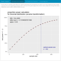
Power Analysis / Sample size calculation II. Proportions.
Power analysis is the statistical procedure used to determine if a test contains enough power to reach an acceptable conclusion. "Power" is the probability of detecting a “true” effect, when the effect exists. A common mistake made by many is to use statistical methods meant for continuous variables on discrete count variables. Proportions are derived from events that can be classified as either successes or failures, i.e. a proportion is a simple ratio of counts of success to counts of failures. In scientific settings, for example, you may ask: What proportion of cells express a specific antigen and does an experimental treatment cause that proportion to change? The purpose of conducting power calculations a priori is to determine the number of trials, or subjects or sample size, to use for the study you wish to conduct and hence to be able to forecast the funding needed to carry out an experiment. In non-scientific settings, a practical application would be that of a casino trying to make sure there is no small bias in the dice purchased that could be used by a player to gain an advantage against the house: Power analysis indicates how many rolls are needed to detect a bias.
Source: Emory University, Department of Pharmacology and Chemical Biology, School of Medicine / Michigan Technological University – Applied Cognitive Science and Human Factors Program

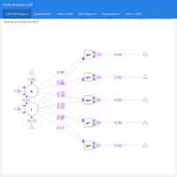
Cognitive Analytics / Psychometrics: IRT Item Response Theory. Case study: Law School Admission Test (LSAT)
A (standardized) knowledge test consists of a set of questions / a directional scale used to discriminate people based on some psychometric property. For instance, you might want to know whether an individual question is good at separating your tested population into two groups (regardless of difficulty) or you might want to design appropriate tests optimizing item discriminability.
Under the umbrella of test theory, Item Response Theory (IRT) aims at testing people (for example, students) and derives the probability of each response as a function of parameters. The assumption is that of underlying traits or dimensions you are measuring based on data consisting mostly of categorical, dichotomous, polytomous or ordered predictors. The simplest binary IRT model (Rasch model) has only one item difficulty parameter and indicates the probability of a correct response as a function of the individual ability given the single item difficulty parameter. The 2PL or 2-parameter logistic has two parameters: person (a person's ability) and item (how good the item is at figuring a person out). In a 3PL or 3-parameter logistic, you would incorporate a guessing parameter to estimate how easy an item is to be guessed.
The LSAT is a classical example in educational testing for ability traits and was designed to measure a single latent ability scale. This dataset comprises responses of 1000 individuals to 5 questions.
Source: Harrisburg University of Science and Technology, Cognitive Analytics
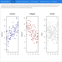
Mixture Models: Mixture of Regressions II. Case study: Predicting student performance
A mixture model is a probabilistic model for representing the presence of sub-populations within an overall population, when the data does not identify the sub-population to which an individual observation belongs to. Expectation-Maximization is an iterative process whereby you apply two complementary processes in the case of a population where you have each sub-group defined by a linear model.
Example: A longitudinal study was conducted to measure student learning ability over time. After repeated testing, maybe some get fatigued and so their data get worse over time, while others learn and so their data get better over time. On average, the performance may be flat, but this could hide two separate groups. If data is not labeled, they may not be easily detectable. If you knew what type of student each subject was, you would be able to fit separate regression models, but as you don’t, a mixture modelling approach can be handy.
Source: Michigan Technological University – Applied Cognitive Science and Human Factors Program
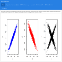
Mixture Models: Mixture of Regressions I. Case study: Predicting group belonging
A mixture model is a probabilistic model for representing the presence of sub-populations within an overall population, when the data does not identify the sub-population to which an individual observation belongs to. Expectation-Maximization is an iterative process whereby you apply two complementary processes in the case of a population where you have each sub-group defined by a linear model.
Example: A study comprising two types of people was conducted on a movie rating site to measure how romantic they are: those who like romantic comedy movies, and those who hate romantic comedies. As you would expect, there is a crossing pattern in the data. If you knew what type of person each person was, you would be able to fit separate regression models, but as you don’t, you can try a mixture modelling approach.
Source: Michigan Technological University – Applied Cognitive Science and Human Factors Program
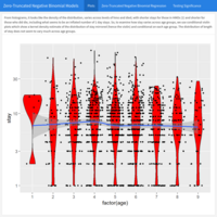
Count Regression Models III: Zero-Truncated Negative Binomial Model. Case study: Predicting length of hospital stay
Zero-truncated negative binomial regression is used to model count data for which the value zero cannot occur and for which overdispersion exists. It is not recommended that negative binomial models be applied to small samples.
Example: A study comprising 1,493 observations of length of hospital stay (in days) is modeled as a function of age, kind of health insurance and whether or not the patient died while in the hospital. Length of hospital stay is recorded as a minimum of at least one day.
Source: UCLA University of California, Los Angeles – Advanced Research Computing, Statistical Methods and Data Analytics
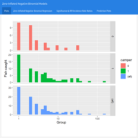
Count Regression Models II: Zero-Inflated Negative Binomial Model. Case study: Prediction of fish caught.
Zero-inflated negative binomial regression models count outcome variables with excessive zeros and are usually appropriate for over-dispersed count responses. Zero-inflated Poisson Regression would do better when the data are not over-dispersed, i.e. when variance is not much larger than the mean. Ordinary Count Models like Poisson or negative binomial models might be more appropriate if there are not excess zeros. It is not recommended that zero-inflated negative binomial models be applied to small samples.
Example: Wildlife biologists want to model how many fish are being caught by fishermen at a state park. Visitors are asked how long they stayed, how many people were in their group, if there were any children in the group, how many fish were caught, and whether or not they brought a camper to the park. Some visitors do not fish, but there is no data on whether a person fished or not. Some visitors who did fish did not catch any fish so there are excess zeros in the data because of the people that did not fish. This case exemplifies a perfect use of ZINB models where the zero outcome is due to two different processes: a subject has gone fishing vs. not gone fishing. If not gone fishing, the only outcome possible is zero. If gone fishing, it is then a count process. The two parts of the a zero-inflated model are a binary model, usually a logit model to model which of the two processes the zero outcome is associated with and a count model, in this case, a negative binomial model, to model the count process.
Source: UCLA University of California, Los Angeles – Advanced Research Computing, Statistical Methods and Data Analytics
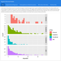
Count Regression Models I: Negative Binomial Model. Case study: Prediction of absence days
Negative binomial regression is appropriate for modeling over-dispersed count outcome variables. A common cause of over-dispersion is excess zeros by an additional data generating process. In this situation, a zero-inflated regression model should be considered. But, if the data generating process does not allow for any 0s (for instance, number of days spent in the hospital), then a zero-truncated model may be more appropriate. It is not recommended that negative binomial models be applied to small samples.
Example: Attendance behavior of 314 high school juniors at two schools. Predictors of days of absence are the type of program the student is enrolled in (vocational, general or academic) and a standardized math test score.
Source: UCLA University of California, Los Angeles – Advanced Research Computing, Statistical Methods and Data Analytics
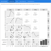
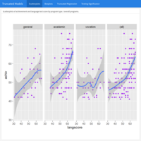
Censored and Truncated Regression Analysis III: Interval Models. Case study: Prediction of academic achievement
A generalization of censored regression, interval regression, is used to model outcomes that have interval censoring. In such cases, the ordered category into which each observation falls is known, but not the exact value of the observation.
Example: Prediction of GPA scores from teacher ratings of effort, writing test scores and the type of program in which the student was enrolled (vocational, general or academic). In these 30 observations, the GPA score is represented by two values: the lower interval score and the upper interval score. The writing test scores, the teacher rating and the type of program (a nominal variable which has three levels) are write, rating and type, respectively.
Source: UCLA University of California, Los Angeles – Advanced Research Computing, Statistical Methods and Data Analytics
Censored and Truncated Regression Analysis II: Truncated Models. Case study: Academic achievement
Truncated regression is used to model dependent variables for which some of the observations are not included in the analysis because of the value of the dependent variable. Note that with truncated regression, the variance of the outcome variable is reduced compared to the distribution that is not truncated. Also, if the lower part of the distribution is truncated, then the mean of the truncated variable will be greater than the mean from the untruncated variable; if the truncation is from above, the mean of the truncated variable will be less than the untruncated variable.
Example: A study of students in a special gifted and talented education program wishes to model achievement as a function of language skills and the type of program in which the student is currently enrolled. A major concern is that students are required to have a minimum achievement score of 40 to enter the special program. Hence the sample is truncated at an achievement score of 40.
Source: UCLA University of California, Los Angeles – Advanced Research Computing, Statistical Methods and Data Analytics

Censored and Truncated Regression Analysis I: Tobit Models. Case study: Academic aptitude
The Tobit Model or censored regression model estimates linear relationships between variables when there is either left- or right-censoring in the dependent variable (also known as censoring from below and above, respectively). Censoring from above: when cases with a value at or above some threshold, all take on the value of that threshold, so that the true value might be equal to the threshold (but it might also be higher). Censoring from
below: values that fall at or below some threshold are censored.
Example: Measure of academic aptitude (scaled 200-800) to be modeled using reading and math test scores, as well as the type of program the student is enrolled in (academic, general, or vocational). The problem here is that students who answer all questions on the academic aptitude test correctly receive a score of 800 max., even though it is likely that these students are not all truly equal in aptitude. The same is true of students who answer all of the questions incorrectly: they would all have a score of 200, although they may not be of equal aptitude.
Source: UCLA University of California, Los Angeles – Advanced Research Computing, Statistical Methods and Data Analytics
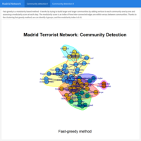
Social Network Analytics II. Case study Terrorist attack in Madrid, 2004
In this example, the terrorist (undirected) network behind the Madrid train bombing in 2004 is investigated based on the connections between the terrorists. If a network has a community structure, then it is possible to assign vertices to unique sets. Within each set of vertices, the connections between members will be more dense than the connections between different sets of vertices. Particularly in large networks like this one, it helps us identify functional subunits. In this section, two algorithms were used to detect communities: Fast-greedy vs. edge-betweenness.
Source University of Barcelona, University of Udine

Social Network Analytics I. Case study: Terrorist attack in Madrid, 2004
Many different patterns of relationships between individuals/entities may be illustrated as a social network with the help of a sociogram depicting their interconnections. The presence or absence of each interconnection indicates whether there exists some form of relationship between each pair of parties and they may represent, for instance, friendships between individuals, flight routes between cities, money transfer between an originator and a beneficiary, etc. In this example, the terrorist (undirected) network behind the Madrid train bombing in 2004 is investigated based on the connections between the terrorists: trust or friendship, links to Al Qaeda and Osama Bin Laden, co-participation in training camps or wars, and co-participation in previous terrorist attacks. Includes: transitivity, density, triads, cliques, eigenvector centrality plot.
Source: University of Barcelona, University of Udine

Necessary Condition Analysis (NCA) - Case Study: Allowing high life expectancy
NCA is based on necessity causal logic and aims to describe the expected causal relationships between different concepts. If a certain level of the condition is not present, a certain level of the outcome will not be present. Other factors cannot compensate for the missing condition. The necessary condition allows the outcome to exist, but does not produce it. This is different from sufficiency causal logic where the condition produces the outcome.
This analysis tests a first hypothesis that vaccination is necessary for life expectancy, i.e. a high level of vaccination of a country's population is a necessary condition for a country's high level of life expectancy. A second hypothesis to be tested is that the basic education of a country's population is a necessary condition for its life expectancy. This is because basic education relates to health and safety as it enables a basic understanding of healthy food, sanitation, clean water, safety and traffic, among many other aspects.
Source: Erasmus University – Rotterdam School of Management, Department of Technology and Operations Management
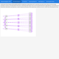
Factor Analysis (FA) IV: Latent Growth Models (LGM)
Factor Analysis (FA) encompasses a set of measurement models such as Exploratory Factor Analysis (EFA), Confirmatory Factor Analysis (CFA), Structural Equation Modeling (SEM), and Latent Growth Models (LGM). A construct is a hypothesized attribute or factor that can't be directly observed or measured.
Latent Growth Models (LGM) extend the capacities of Factor Analysis models to allow for the investigation of longitudinal trends or group differences, introducing measurement invariance as a way to assess the plausibility of stratifying the CFA model into distinctive units of analysis.
Source of the data: UCLA University of California, Los Angeles – Advanced Research Computing, Statistical Methods and Data Analytics
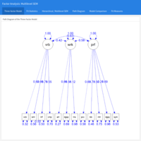
Factor Analysis (FA) III.I: Multilevel Structural Equation Modeling (SEM)
In this analysis, the previous SEM analysis is extended to a multilevel model, where General IQ is the reason for the subscores on the WAIS-III IQ Scale (Wechsler Adult Intelligence Scale version III).

Factor Analysis (FA) III: Structural Equation Modeling (SEM)
Factor Analysis (FA) encompasses a set of measurement models such as Exploratory Factor Analysis (EFA), Confirmatory Factor Analysis (CFA), Structural Equation Modeling (SEM), and Latent Growth Models (LGM). A construct is a hypothesized attribute or factor that can't be directly observed or measured. Examples of commonly studied constructs include self-determination, reasoning ability, IQ, political affiliation, and extraversion.
Structural equation modeling (SEM) is a linear model framework that models both simultaneous regression equations with latent variables, with the following possible relationships:
• observed to observed variables (e.g. regression)
• latent to observed variables (e.g. confirmatory factor analysis)
• latent to latent variables (e.g. structural regression)
SEM uniquely encompasses both measurement and structural models. The measurement model relates observed to latent variables and the structural model relates latent to latent variables.
Source of the data: datacamp
Factor Analysis (FA) II: Confirmatory Factor Analysis (CFA)
Factor Analysis (FA) encompasses a set of measurement models such as Exploratory Factor Analysis (EFA), Confirmatory Factor Analysis (CFA), Structural Equation Modeling (SEM), and Latent Growth Models (LGM). A construct is a hypothesized attribute or factor that can't be directly observed or measured. Examples of commonly studied constructs include self-determination, reasoning ability, IQ, political affiliation, and extraversion.
CFA is used to evaluate the strength of the hypothesized relationships between items and the constructs they were designed to measure (for instance, extraversion). Instead of letting the data tell us the factor structure as with EFA, in CFA we pre-determine the factor structure and verify the psychometric structure of a previously developed scale.
Source of the data: psych R package & datacamp

Factor Analysis (FA) I: Exploratory Factor Analysis (EFA)
Factor Analysis (FA) encompasses a set of measurement models such as Exploratory Factor Analysis (EFA), Confirmatory Factor Analysis (CFA), Structural Equation Modeling (SEM), and Latent Growth Models (LGM). A construct is a hypothesized attribute or factor that can't be directly observed or measured. Examples of commonly studied constructs include self-determination, reasoning ability, IQ, political affiliation, and extraversion.
EFA is used during measure development to explore factor structure and determine which items do a good job of measuring the construct (for instance, IQ).
Source of the data: psych R package & datacamp

Descriptive Analytics: Interactive Dashboard
Publicly available dataset from a bike share service in the San Francisco area, USA. The dataset has records for all bike trips taken from station to station with locations and times.

Survival Analysis - Case study: lung cancer patients
For the purpose of this analysis, data describing survival of patients with advanced lung cancer is used (source: survival package). The survival time (in days), status (censored or dead), age (in years), the patient's sex, and weight loss (pounds) in the last 6 months are indicated. Techniques used: Kaplan-Meier estimator of the survival function, (stratified) Cox proportional hazards model.
Source: UCLA Office of Advanced Research Computing, Statistical Methods and Data Analytics
Spatial Analysis - Case study: Multi-dimensional Index mapping for Liverpool, UK
Multi-Dimensional indices are used to create many different data sets as a form of composite descriptive analysis. Based on the insights they provide, more sophisticated analyses may follow. In this case, the AHAH index (or Access to Healthy Assets & Hazards) was developed to measure how ‘healthy’ neighbourhoods are. It combines indicators under four different domains of accessibility:
Retail services (access to fast food outlets, pubs, off-licences, tobacconists, gambling outlets),
Health services (access to GPs, hospitals, pharmacies, dentists, leisure services),
Physical environment (Blue Space, Green Space - Passive), and
Air quality (Nitrogen Dioxide, Particulate Matter 10, Sulphur Dioxide).
Census data for Liverpool Lower Layer Super Output Areas, 2011, as well as Access to Healthy Assets & Hazards (AHAH) multi-dimensional index input datasets come from the CDRC Data website.
Source of the data: UK Consumer Data Research Centre
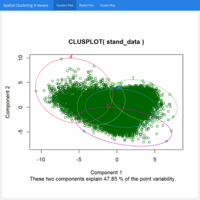
Spatial Analysis - Case study: Geodemographic classification: Clustering using k-means, Greater London, UK
The goal of this analysis is to classify Greater London areas based on their demographic characteristics into 5 clusters using the k-means clustering algorithm.
Output area boundaries for London shapefile as of 2011 as well as Census variables at the Output Area level for the UK come from the CDRC Data website.
Source of the data: UK Consumer Data Research Centre
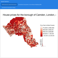
Spatial Regression Analysis - Case study: Interpolation of point data, borough of Camden, London, UK / Part III
Interpolation describes a means of estimating a value for a particular setting based on a known sequence of data. In a spatial context, it refers to using an existing distribution of data points to predict values across space, including in areas where there are little to no data. One of the most commonly used interpolation methods is Inverse Distance Weighting (IDW). While IDW is created by looking at just known values and their linear distances, kriging also considers spatial autocorrelation; therefore, it is more appropriate if there is a known spatial or directional bias in the data.
Census data pack for Local Authority District Camden as of 2011 come from the CDRC Data website.
Source of the data: UK Consumer Data Research Centre
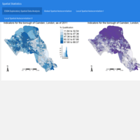
Spatial Regression Analysis - Case study: Geographically Weighted Regression, borough of Camden, London, UK / Part II
The aim of this analysis is to determine whether Qualification (the dependent variable) is associated with Unemployment and White British population rates in Camden, London. Geographically Weighted Regression (GWR) describes a family of regression models in which the coefficients are allowed to vary spatially.
Census data pack for Local Authority District Camden as of 2011 come from the CDRC Data website.
Source of the data: UK Consumer Data Research Centre
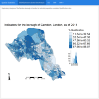
Spatial Analysis - Case study: Clustering in the borough of Camden, London, UK / Part I
The aim of this analysis is to determine whether qualification and White British population rates cluster in Camden, London. Spatial autocorrelation measures how distance influences a particular variable. In other words, it quantifies the degree of which objects are similar to nearby objects. Variables are said to have a positive spatial autocorrelation when similar values tend to be nearer together than dissimilar values. In population data this is often the case as persons with similar characteristics tend to reside in similar neighbourhoods due to a range of reasons including house prices, proximity to workplaces and cultural factors.
Census data pack for Local Authority District Camden as of 2011 come from the CDRC Data website.
Methods used include the following: distance based connectivity (features within a given radius are considered to be neighbors), global / local spatial autocorrelation (Moran’s I), static / interactive maps.
Source of the data: UK Consumer Data Research Centre

Spatial Accessibility - Case study: Spatial access to full service banks in the City of Los Angeles, CA
Spatial accessibility refers to the ease with which residents of a given neighborhood can reach amenities. Specifically, low-income and majority-minority neighborhoods may be spatially inaccessible to a nearby financial institution, with the consequences that such situation implies.
Census tract polygon features and racial composition data come from the 2015-2019 American Community Survey (the US Census). Full-service banks and credit unions data of 2020 in Los Angeles come from the Federal Deposit Insurance Corporation and from the National Credit Union Administration.
To estimate spatial accessibility, the following methods were used: Points-in-polygon, buffer analysis , (euclidean) distance to nearest amenity, and Two-step Floating Catchment Area.
Source of the data: UC Davis - Department of Human Ecology, Community and Regional Development, USA
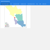
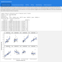
Spatial Econometrics: Spatial Heterogeneity - Case study: Housing values in the San Francisco Bay Area, USA
This analysis answers the following questions: What socioeconomic and built environment characteristics are associated with housing values in the Bay Area? Do these relationships vary across Bay Area regions? The Bay Area is composed of nine counties, categorized as: East Bay (Alameda and Contra Costa), North Bay (Marin, Napa, Solano and Sonoma), South Bay (Santa Clara), Peninsula (San Mateo) and San Francisco. Data come from a Bay Area census tract shapefile (2013-2017 American Community Survey, the United States Census).
Several types of spatial regression models are included: Interaction model, Stratified model, Spatial regime model, and Geographically Weighted Regression model.
Source of the data: UC Davis - Department of Human Ecology, Community and Regional Development, USA
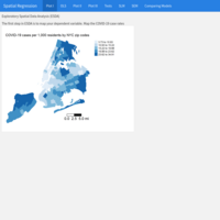
Spatial Statistics: Spatial Regression - Case study: COVID-19 case rates in New York City, USA
The goal of this analysis is to examine the relationship between neighborhood socioeconomic and demographic characteristics and COVID-19 case rates in New York City when COVID was first detected in the United States (2020). Data come from a shape file containing COVID-19 cases per 1,000 residents and demographic and socioeconomic characteristics for New York city zip codes. COVID-19 case data come from the NYC Department of Health and Mental Hygiene (confirmed cases up through May 1, 2020). Socioeconomic and demographic data were downloaded from the 2014-2018 American Community Survey, the United States Census.
Two standard types of spatial regression models are included: a spatial lag model (SLM), which models dependency in the outcome, and a spatial error model (SEM), which models dependency in the residuals. Robust versions of the Lagrange Multiplier Tests were used to determine the appropriate model.
Source of the data: UC Davis - Department of Human Ecology, Community and Regional Development, USA

Spatial Statistics / Principal Components Analysis - Case study: Neighborhood concentrated disadvantage index for Sacramento, CA.
The goal of this analysis is to create a neighborhood concentrated disadvantage index for the Sacramento Metropolitan Area. One of the methods for creating indices is Principal Components Analysis (PCA). The data come from the 2015-2019 American Community Survey (Census) using two measures of neighborhood health: the 2017 crude prevalence of residents aged 18 years and older reporting that their mental health is not good and the 2017 crude prevalence of diagnosed diabetes among adults aged >= 18 years. This data come from the Center for Disease Control and Prevention (CDC) 500 cities project, which uses the Behavioral Risk Factor Surveillance System (BRFSS) to estimate tract-level prevalence of health characteristics.
Source of the data: UC Davis - Department of Human Ecology, Community and Regional Development, USA

Spatial Statistics: Spatial Regression - Case study: Tract-level (census) prevalence of health characteristics in Seattle, WA
The goal of this analysis is to examine the relationship between neighborhood socioeconomic and demographic characteristics and the prevalence of poor health at the neighborhood level in Seattle, WA. The dependent variable is a measure of the 2017 crude prevalence of residents aged 18 years and older reporting that their health is not good. Data come from the Center for Disease Control and Prevention (CDC) 500 cities project, which uses the Behavioral Risk Factor Surveillance System (BRFSS) to estimate tract-level prevalence of health characteristics. Census data for Seattle comes from the American Community Survey, the United States Census.
Two standard types of spatial regression models are included: a spatial lag model (SLM), which models dependency in the outcome, and a spatial error model (SEM), which models dependency in the residuals.
Source of the data: UC Davis - Department of Human Ecology, Community and Regional Development, USA

Spatial Statistics - Case study: Neighborhood housing eviction rates in Sacramento, California
The goal of this analysis is to determine whether eviction rates cluster in Sacramento, CA. The main dataset is a shapefile containing 2016 court-ordered house eviction rates for census tracts in the Sacramento Metropolitan Area. Techniques applied: distance based connectivity (features within a given radius are considered to be neighbors), global / local spatial autocorrelation (Moran’s I, Getis-Ord), static maps / interactive mapping (Leaflet / OpenStreetMap). Source of the data: UC Davis - Department of Human Ecology, Community and Regional Development, USA
Spatial Econometrics: From simple OLS regression to Spatial Multilevel Modelling. Part II
The objective of this analysis is to explore if there is variation in the relationship between unemployment rate and the proportion of population in long-term illness. 8 MSOAs containing OAs with the highest unemployment rates in Liverpool were selected. Furthermore, an example of centering is introduced to build and then compare different models to find the one that fits the data better.
Source of the data: University of Liverpool, United Kingdom
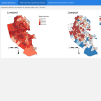
Spatial Econometrics: From simple OLS regression to Spatial Multilevel Modelling. Part I
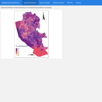
The objective of this analysis is to understand the spatial distribution of the proportion of unemployed population in Liverpool, and why and where concentrations in this proportion occur. Observations nested within higher geographical units may be correlated; hence, caring about the structure of the data is important in order to draw correct statistical inference, link context to individual units, and help mitigate the effects of spatial autocorrelation.
Data for Liverpool from England’s 2011 Census (Office of National Statistics), comprising selected variables capturing demographic, health and socio-economic attributes of the local resident population at four geographic levels: Output Area (OA), 298 Lower Super Output Area (LSOA), 61 Middle Super Output Area (MSOA) and Local Authority District (LAD).
The data (1584 observations) are hierarchically structured: OAs nested within LSOAs, LSOAs nested within MSOAs, and MSOAs nested within LADs. The average of nested OAs within LSOAs is 5 and within MSOAs is 26.
Source of the data: University of Liverpool, United Kingdom

Multilevel Generalized Linear Model. Case Study: College Basketball Referees - Comparing Logistic Regression with Multilevel Modeling.
Some questions this model answers: Is there evidence that referees tend to “even out” foul calls when one team starts to accumulate more fouls? Is the score differential associated with the probability of a foul on the home team? Is the effect of foul differential constant across all foul types during these games?
For this dataset with about 5000 observations spanning the period 2009-2010, a logistic regression model with interactions is compared to a multilevel generalized linear model with cross-random effects. Confidence intervals applying bootstrapping were used to compare full and reduced models that differ in their variance components and a final multilevel model was selected.
This analysis shows that a multilevel regression model with cross-random effects outperforms a logistic regression model with interactions (based on AIC/BIC, both lower for the multilevel version), and also gives a sense of the different fixed effects significance as well as their magnitudes when both are compared. Furthermore, it shows that adding random effects allows for more precise conclusions because it takes into account correlation structures in the data.
Source of the data: St. Olaf College, USA
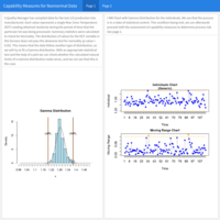
Process & Quality Improvement / Six Sigma: Statistical Process Control - Control Charts for Nonnormal Data
X and Moving Range charts are used when the process changes too slowly in repeated measures, when measures are extremely homogenous, or when individual values do not fall into logical subgroups, and when measures are expensive as with destructive testing.
Example: A Quality Manager has recently installed a new furnace, and has randomly measured the temperature in the rear zone of the furnace. We'll assess Statistical Process Control and Process Capability indices.
Source of the data: University of Colorado Boulder
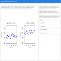
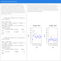
Process & Quality Improvement / Six Sigma: Statistical Process Control - Control Charts for Discrete Data
The Vice-President of Marketing at a large metals company wants to analyze performance in the Inside Sales Department. One of the most common problems in this area is the number of calls that were never answered, resulting in the customer giving up, hanging up, and probably calling their competitor.
Period 1 corresponds to the initial data collected on “Dropped Calls” from a total of 250 calls received during the same time of day, for 70 randomly selected days and times for a number of weeks. Additional data were collected (Period 2). The Problem Solving Team was tasked with the generation of improvement oriented activities, and we are going to assess those results using Statistical Process Control techniques and p charts.
Source of the data: University of Colorado Boulder
Process & Quality Improvement / Six Sigma: Statistical Process Control - Control Charts for Discrete Data
Attribute charts like the c chart will reflect data that comes from a Poisson distribution and typically represent an absolute count, such as the number of errors per unit or interval.
Example: Automobile Assembly plant where a complex fuel tank / sensor / bracket assembly is built and placed into vehicles. At a random time each day, 5 consecutive assemblies are selected from the assembly line and the inspector counts the total number of defects (Assembly Errors) found in the group of the 5 units selected. There are two periods applicable to the data: before and after a training program was instituted. With the help of control charts and appropriate statistical tests, we can demonstrate that the training indeed results in an improvement in performance.
Source of the data: University of Colorado Boulder
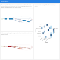
Process Improvement / Process Mining: Process map, performance map, precedence matrix
Efficient processes are one of the main components of successful organizations. Process mining uses data science to bridge the gap between the process models that were used to configure a system, and the event data that was recorded in the system. By analyzing this data, we can get insights and suggest process improvements. For instance, the process model can be overlaid with performance information to show bottlenecks. Example: Emergency Room of a hospital providing the required services to screen, examine, and take care of patients in the most effective way.
Source of the data: bupaR library
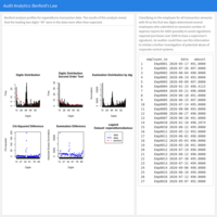
Audit / Forensic Analytics: Benford’s Law to spot anomalies
Benford’s law states that a simple comparison of first-digit frequency distribution from the data with the expected distribution ought to show up any anomalous results. Under certain conditions, an analysis of the frequency distribution of the first or second digits can detect abnormal patterns in the data and may identify possible fraud.
Example: Over 330 transactions ranging from $8 to $1'600 carried out by 16 employees in 2020 were analyzed for possible anomalies.
Source of the data: Department of Information & Decision Sciences, University of Illinois, Chicago, IL, USA

Process Improvement / Six Sigma: Control phase of the DMAIC cycle: Individual and Moving-Range (I/MR) and X¯(x bar) – R Charts
Process Control Charts are two-dimensional charts that represent the variables to be monitored. The values of the characteristic are plotted sequentially in the order in which they have arisen. Depending on the type of data to be analyzed, these values can be individual values or group means. For continuous variables (for example, humidity), the moving average chart and the x bar chart monitor the process location over time and allow to uncover small shifts in the process mean.

Process Improvement / Six Sigma: Measure phase of the DMAIC cycle: Pareto analysis
A Pareto Analysis can be used when we have to prioritize a list of elements, such as the causes of failure in our process, in order to differentiate between the “vital few” (20%) and the “useful many” (80%). Example : Construction company investigating why a sampling of deadlines on projects developed in the last 2 years went unfulfilled. It also estimated the cost of these delays for the company (larger labor force, extra payments, etc.). The next step is to find the causes responsible for 80% of the effect.

Process Improvement / Six Sigma: Measure phase of the DMAIC cycle: cause-and-effect diagram
After describing the process with a process map, where we have identified the parameters that influence the features of the process, we have an overview of the parameters that can engender problems with the process. With the help of brainstorming, six Ms, five whys, etc., we can identify the causes of errors that may arise in the process and group the causes into categories on several levels. Example: construction project.

Process Improvement / Six Sigma: Measure Phase of the DMAIC cycle: Process Capability Analysis
In this example from a winery, the actual volume in a 20-bottle sample was measured after the filling process. We compare the customer specifications with the performance of the process. They are based on the fact that the natural limits or effective limits of a process are those between the mean and ±3 standard deviations (sigma). The results show that the capability index (1.547) is quite acceptable, though it can be improved to reach the desired 1.67 value. Furthermore, the estimation of the long-term sigma indicates that we could have problems if the long-term variation turns out to be much higher than the short-term one.
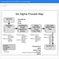
Process Improvement / Quality Management: Six Sigma in Action - Define phase of the DMAIC cycle
The Six Sigma methodology consists of the application of the scientific method to solve problems and improve processes. When Six Sigma is implemented, it follows the DMAIC cycle, which can be defined as: Define, Measure, Analyze, Improve, and Control. Example of a process map for a restaurant.
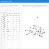
Prescriptive Analytics: Performance Evaluation. Data Envelopment Analysis (DEA) for Modeling marketing efficiency using optimization algorithms (linear programming).
An auto industry producer needs to understand the efficiency of its marketing strategy. There are marketing expenses associated with several advertising channels and for each brand we have the total number of cars sold.
Some questions this model answers: Can marketing spending be reduced? Is “Digital” the best marketing channel? How should resource allocation be changed in order to become more efficient? What is the best channel to optimize marketing efforts? How can we maximize sales / minimize costs?
Source of the data: International Laboratory for Applied Network Research, National Research University Higher School of Economics, Moscow, RU
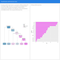
Predictive Analytics: Machine Learning. Classification with decision trees
Predicting animal classes based on different attributes using the rpart algorithm trained with optimal hyperparameter combination.
Source of the data: mlbench library
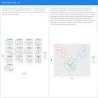
Predictive Analytics: Machine Learning. Classification using LDA and QDA
Classification of a contaminated wine sample using Linear Discriminant Analysis (LDA) and Quadratic Discriminant Analysis (QDA). The objective is to predict which of 3 different vineyards the spoiled bottle came from.
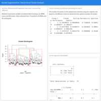
Predictive Analytics: Machine Learning. Cluster Analysis in Marketing Research: Market Segmentation
Application of the hierarchical clustering algorithm using the ward distance method and attribute importance weights considered by students when buying a car.
Source of the data: Columbia University, NY
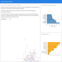
Predictive Analytics: Machine Learning. Market Basket Analysis (Association Rules Mining) (interactive)
Apriori algorithm applied to analyze 9'800 transactions of grocery shopping data mainly to determine lift. Rules plot, most / least frequent items.
Source of the data: apriori library

Predictive Analytics: Statistical Analysis + Machine Learning. Forecasting (interactive)
Some basic forecasting models were developed and evaluated: ARIMA, Exponential Smoothing, Linear Regression, and MARS (Multivariate Adaptive Regression Splines).
Source of the data: M Open Forecasting Center (MOFC), the 750th Monthly Time Series used in the M4 Competition, Modeltime ecosystem (Business Science.io)
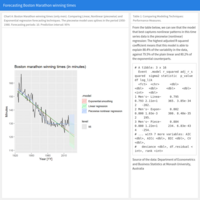
Predictive Analytics: Statistical Analysis. Forecasting Boston marathon
Forecasting Boston marathon winning times (only men). Comparing Linear, Nonlinear (piecewise) and Exponential regression forecasting techniques.

Predictive Analytics: Statistical Analysis. Forecasting Australian Tourism (hierarchical and grouped forecasts)
Coherent 2 year-Forecasts of overnight trips for Australia using bottom-up, ordinary least squares, and minimum trace optimal reconciliation techniques.
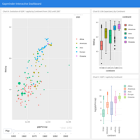
Descriptive Analytics: Gapminder Interactive Dashboard
Gapminder provides values for life expectancy, GDP per capita, and population, every five years, from 1952 to 2007 for 142 countries