tkubota0720
Takafumi Kubota
Recently Published

suzuki_6785_week2
suzuki_6785_week2


spotify03
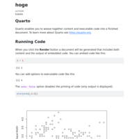
Spotify’s vast streaming catalog offers an ideal sandbox for probing how musical style interacts with commercial success. This technical report chronicles the assembly of an analysis-ready dataset that merges two complementary slices—“High Popularity” and “Low Popularity”—from the Kaggle Spotify Music Data repository. After appending a categorical popularity label, we condense over thirty playlist-level genre tags into six headline genres to streamline visualisation and modelling. Duplicate records are systematically flagged at the track-artist-playlist axis using flexible separator rules that detect comma, ampersand, and semicolon delimiters within multi-artist fields. Because Spotify sometimes assigns the borderline popularity score of sixty-eight to both classes, ambiguous low-popularity rows are excluded to guarantee mutually exclusive groups. The resulting table contains 13,342 unique tracks spanning electronic, pop, Latin, hip-hop, ambient, rock, and an aggregated “others” bucket. Every transformation is fully scripted in R and encapsulated within a Quarto document, enabling frictionless reruns on fresh dumps or forked datasets. The cleaned corpus supports subsequent inquiries into genre-specific audience reach, collaboration networks, and the quantitative drivers of streaming attention. Practitioners can reuse the workflow as a drop-in template for playlist analytics, while researchers gain a transparent foundation for reproducible music-industry studies. The code is concise, documented, and easily shareable.

spotify02
This notebook enriches a cleaned Spotify track list with artist-country metadata to support geographic analyses of streaming popularity. Starting from spotify_data_rmdup.csv—a 13 k-row table of unique tracks and curated audio-features—we query the public MusicBrainz API in 1 000-row batches, assigning one or more ISO-3166 country codes to every artist credited on each track. A lightweight in-memory cache plus an on-disk RDS file prevent redundant requests, while an adjustable one-second delay respects MusicBrainz rate limits. All steps—chunk creation, safe API calls, duplicate handling, progress reporting, and final export—are fully scripted in R and wrapped in a Quarto document for reproducibility. The resulting file, dat_with_country_all.rds, adds a pipe-delimited country field that can be merged back into genre or popularity studies, enabling questions such as “Which countries dominate high-popularity electronic playlists?” or “How do cross-border collaborations affect reach?” Researchers can reuse or extend the workflow with minimal edits.

spotify01
Spotify’s vast streaming catalog offers an ideal sandbox for probing how musical style interacts with commercial success. This technical report chronicles the assembly of an analysis-ready dataset that merges two complementary slices—“High Popularity” and “Low Popularity”—from the Kaggle Spotify Music Data repository. After appending a categorical popularity label, we condense over thirty playlist-level genre tags into six headline genres to streamline visualisation and modelling. Duplicate records are systematically flagged at the track-artist-playlist axis using flexible separator rules that detect comma, ampersand, and semicolon delimiters within multi-artist fields. Because Spotify sometimes assigns the borderline popularity score of sixty-eight to both classes, ambiguous low-popularity rows are excluded to guarantee mutually exclusive groups. The resulting table contains 13,342 unique tracks spanning electronic, pop, Latin, hip-hop, ambient, rock, and an aggregated “others” bucket. Every transformation is fully scripted in R and encapsulated within a Quarto document, enabling frictionless reruns on fresh dumps or forked datasets. The cleaned corpus supports subsequent inquiries into genre-specific audience reach, collaboration networks, and the quantitative drivers of streaming attention. Practitioners can reuse the workflow as a drop-in template for playlist analytics, while researchers gain a transparent foundation for reproducible music-industry studies. The code is concise, documented, and easily shareable.

Social Isolation yearly changes
This study examines changes in time allocation across activities from 2006 to 2021, focusing on relationships such as being alone, with family, colleagues, or others. The findings show an increase in time spent alone and a decline in interactions with others, particularly non-family members. These trends reflect societal changes like individualism, digitalization, and shifting work-life dynamics. The analysis highlights that secondary activities, such as work, are increasingly done alone, while leisure activities show a sharp decline in interactions outside the family. These results reveal the growing impact of modern lifestyles on social connections and individual behaviors.

Visualization of suicide data in New Zealand (3) - Choropleth map
This report visualizes suicide data in New Zealand for 2023 using choropleth maps to highlight spatial variations across districts. Leveraging R and the ggplot2 package, the study processes and cleans data from official sources, addressing missing and anomalous values to ensure accuracy. Two maps are generated: one depicting the absolute number of suicides and another illustrating suicide rates per 100,000 population. The visualizations reveal significant disparities between regions, identifying high-risk districts that require targeted intervention. These insights aim to inform public health strategies and policy-making to effectively address and mitigate suicide rates across New Zealand.

Visualization of suicide data in New Zealand (2)-2 - Age Group
This report analyzes suicide trends in Aotearoa New Zealand for 2023, focusing on differences across age groups and sexes. Using "Suspected" case data from all ethnic groups, the study employs data cleaning and transformation to ensure accuracy. Utilizing R and ggplot2, the report presents stacked bar charts showing both the number of suicide deaths and rates per 100,000 population across age categories. The findings provide insights for public health officials and policymakers to identify high-risk groups and develop targeted intervention strategies, contributing to efforts to reduce suicide rates and enhance mental health support in New Zealand. (Update for missing data.)

Visualization of suicide data in New Zealand (2) - Age Group
This report analyzes suicide trends in Aotearoa New Zealand for 2023, focusing on differences across age groups and sexes. Using "Suspected" case data from all ethnic groups, the study employs data cleaning and transformation to ensure accuracy. Utilizing R and ggplot2, the report presents stacked bar charts showing both the number of suicide deaths and rates per 100,000 population across age categories. The findings provide insights for public health officials and policymakers to identify high-risk groups and develop targeted intervention strategies, contributing to efforts to reduce suicide rates and enhance mental health support in New Zealand.

Visualization of suicide data in New Zealand (1) - Time series
This study analyzes suspected suicide trends in New Zealand from 2009 to 2023. Using R for data cleaning and visualization, it highlights demographic patterns and annual shifts, offering insights for policymakers and researchers.


Subsetting Method
This note customizes the behavior of the [ operator in R to allow row extraction in the form of df[1:3]. By redefining the [.data.frame method using the S3 system, rows are selected when no column is specified. This customization enables differentiation between row and column selection without affecting other object types.

Type Coercion
Type coercion in R refers to the automatic conversion of elements with different data types into a unified type when combined in a vector. R follows a specific data type hierarchy: character > numeric > integer > logical. This ensures that all elements in a vector have the same type. For example, when a logical (TRUE), numeric (17), and character ("twelve") are combined, all elements are coerced into the character type. Similarly, logical values like TRUE and FALSE are converted to 1 and 0 when combined with numeric values. This process allows R to handle mixed-type data efficiently and consistently. Understanding type coercion is crucial for data manipulation, as it prevents unexpected type changes when processing vectors with diverse elements.

ThreeWhiteSoldiers
This R script analyzes and visualizes selected Nikkei 225 stocks to detect the Three White Soldiers (TWS) pattern, a bullish candlestick formation. Utilizing quantmod for data retrieval, TTR for technical analysis, and dplyr for data manipulation, it downloads one year of historical stock data from Yahoo Finance. The script identifies stocks with a TWS pattern on the most recent trading day and visualizes these patterns by adding vertical orange lines with 0.3 transparency to the charts. This automated approach aids analysts and investors in efficiently spotting bullish signals in stock data.

nikkei225
This R script conducts time series analysis and visualization of selected Nikkei 225 stocks. Utilizing quantmod for data retrieval and dplyr for data manipulation, it fetches one-year historical stock data from Yahoo Finance. The script calculates the most recent and prior year weekdays to ensure accurate trading data. It dynamically generates variables for each stock's data and visualizes them using chartSeries with a clean theme. This streamlined process aids financial analysts and researchers in efficiently analyzing and visualizing stock performance.


Data Cleaning 01
In this study, we present a detailed methodology for cleaning and organizing the data from the Spanish football league. The primary objective is to transform raw match data into a structured and analyzable format, ensuring consistency and accuracy. We employ several data processing techniques using R, including reading raw CSV files, converting team names to their abbreviations, and calculating match results. Our approach involves creating a new dataframe that includes both home and away team perspectives, with additional columns for results and win points. The processed data enables more straightforward analysis for various applications, such as performance analysis, trend identification, and predictive modeling. The effectiveness of our method is demonstrated through a step-by-step transformation of the dataset, ensuring that it is ready for advanced statistical analysis and machine learning applications. This paper contributes to the field by providing a reproducible and scalable data cleaning framework, essential for researchers and analysts working with sports data.

eyesdata
This study demonstrates the use of the VGAM package in R to fit a vector generalized linear model (VGLM) with synthetic data. Data for 1000 individuals, including ocular pressure and age, was generated and transformed to include mean ocular pressure and linear predictors. Binary outcomes for eye conditions were derived using the logitlink function. The vglm function was used to fit the model with leye and reye as responses and op as the predictor, specifying a binomial family with odds ratio. The model matrix was generated to show the data structure.

confint
This study simulates the construction of 95% confidence intervals for the true mean using normally distributed random data. By generating 100 samples of size 30, we compute the confidence intervals and identify those that do not contain the true mean, highlighting them in red. The proportion of intervals containing the true mean is calculated to validate the simulation's accuracy. This approach visually demonstrates the reliability of confidence intervals in estimating population parameters.
Spotify
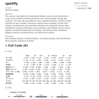
This analysis investigates the relationships between various musical features of songs using a dataset containing attributes such as Danceability, Energy, Key, Loudness, and more. We calculated the mean, standard deviation, and five-number summary for each variable. Correlation matrices were computed, and the most strongly correlated pairs were identified. Boxplots and scatterplot matrices were generated to visualize distributions and correlations. Key findings include a strong negative correlation between Key and Energy, and strong positive correlations between Liveness and Acousticness, and Tempo and Liveness.
100m
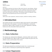
This analysis examines the historical 100m sprint times for male athletes, utilizing linear regression to identify trends over time. A dataset of sprint times from 1964 to 2009 is used to build a regression model, which is then employed to predict sprint times 100 years into the future. The findings include the regression model equation and the predicted sprint time for the year 2109.
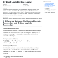
Ordinal Logistic Regression
This study compares multinomial and ordinal logistic regression models using custom penalized error metrics. By applying larger penalties for misordered predictions, the performance of each model is assessed through penalized Mean Absolute Error (MAE) and Mean Squared Error (MSE), highlighting the benefits of considering order in predictive accuracy.
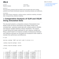
Comparative Analysis of GLM and VGLM Using Simulated Data
This document compares GLM and VGLM using simulated data with multiple predictors and Poisson-distributed responses, evaluating residuals and coefficients.

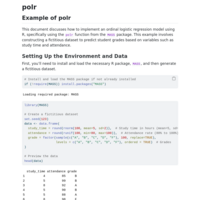
polr
Example of polr


Frequency barchart
R code for the bar chart drawn from the frequency distribution table of the number of party supporters in Figure 1.1 for use in Data Science I classes.

Frequency table
R code to create a frequency table of the number of party supporters in Table 1.1 for use in Data Science I classes.