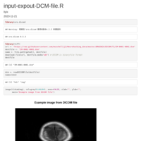
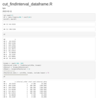
TX-YXL
ASHLEY
Recently Published


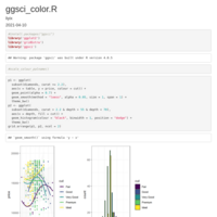
geom_jjtriangle_diagonal heatmap
geom_jjtriangle_diagonal heatmap


gsub-remove-all-string-before-last-two_symbol
"2024-03-18-2024-03-18-data_for_model_05_to_NA-900_XGB_up")
new_strings <- gsub("^.*?_([^_]+)_([^_]+)$", "\\1_\\2", strings)


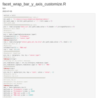


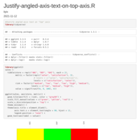
Justify-angled-axis-text-on-top-axis
axis.text
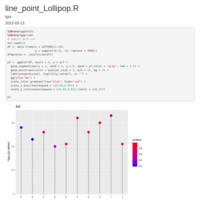
Sankey Diagram
https://app.rawgraphs.io/
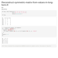
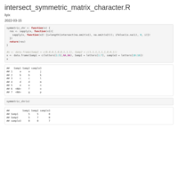
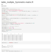
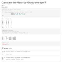
Reconstruct symmetric matrix from values in long-form
df.long <- df.long[df.long$one != df.long$two,]
df <- as.matrix(reshape::cast(df.long, one ~ two, fill=0) )
Circular-heatmap-with-circlize-Plot-area-and-row-labels
col_mat[is.na(col_mat)] <- "gray90"
dend <- set(dend_list,"branches_lty", 3)

chembl_dbi_package
http://ftp.ebi.ac.uk/pub/databases/chembl/ChEMBLdb/latest/
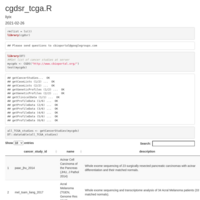
cgdsr_tcga
survival analysis
HEATMAP GGPLOT2
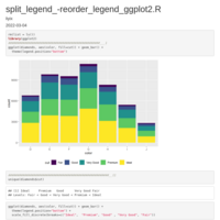
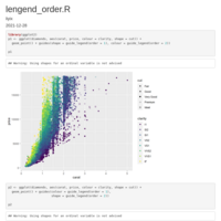
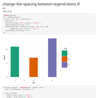
legend title position
axis y text position
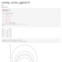
over_circle-example
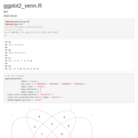
add table
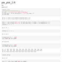
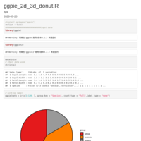
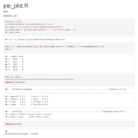
pie_plot_ggplot2
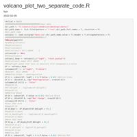
compute_angle = function(perc){
angle = -1
#if(perc < 0.25) # 1st q [90,0]
#angle = 90 - (perc/0.25) * 90
#else if(perc < 0.5) # 2nd quarter [0, -90]
#angle = (perc-0.25) / 0.25 * -90
#else if(perc < 0.75) # 3rd q [90, 0]
#angle = 90 - ((perc-0.5) / 0.25 * 90)
#else if(perc < 1.00) # last q [0, -90]
#angle = ((perc -0.75)/0.25) * -90
if(perc < 0.5) # 1st half [90, -90]
angle = (180 - (perc/0.5) * 180) - 90
else # 2nd half [90, -90]
angle = (90 - ((perc - 0.5)/0.5) * 180)
return(angle)
}
sum_freq = sum(data_6$freq)
secondLevel = data_6 %>%
mutate(running=cumsum(freq), pos=running - freq/2) %>% group_by(1:n()) %>%
mutate(angle=compute_angle((running - freq/2) / sum_freq))
p1 <- ggplot(data_6, aes(x = 1, weight = freq, fill = cancer)) +
geom_bar(width = 1, colour = "black") +
geom_text(x = 1.3, aes(y = centres, label = freq), colour = "black",size = 4) +
scale_fill_manual(values=cancer_col,guide = leg) +
#scale_fill_brewer(palette = c(), direction = -1, guide = leg) +
#scale_color_brewer(palette = "black", direction = 1) +
theme_minimal(base_family = "") +
theme(legend.position = "",
panel.grid.major = element_blank(),
panel.grid.minor = element_blank(),
axis.ticks = element_blank(),
axis.text = element_blank(),
axis.title = element_blank(),
axis.line = element_blank()) +
labs(fill = "", colour = "",
caption = "") +
ggtitle("",
subtitle = "") +
coord_polar(theta = "y",start = 0)
#secondLevel$angle <- -abs(secondLevel$angle)
p1 + geom_text(data=secondLevel, aes(label=paste(period), x=1.5, y=pos, angle=angle,
hjust = c(rep(1, times=8),rep(0,times = 9))))
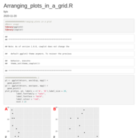
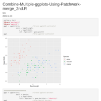
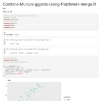
Arranging_plots_in_a_grid
cowplot
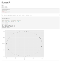
flower
ref: https://mp.weixin.qq.com/s/cAZh-BOMUZH2YI1QQsgpkw
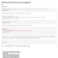
extract all table from PDF
#extract_text() converts the text of an entire file or specified pages into an R character vector.
#split_pdf() and merge_pdfs() split and merge PDF documents, respectively.
#extract_metadata() extracts PDF metadata as a list.
#get_n_pages() determines the number of pages in a document.
#get_page_dims() determines the width and height of each page in pt (the unit used by area and columns arguments).
#make_thumbnails() converts specified pages of a PDF file to image files.
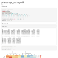
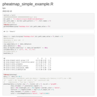
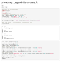
pheatmap_package
tiff(filename = paste0(dir_path,Sys.Date(),"-HP.tiff"),res = 300,
width = 20, height = 20, units = "cm", pointsize = 12,
compression = "lzw",bg = "white")
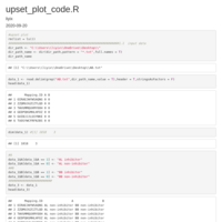
upset_plot_cod
install.packages("UpSetR")
library(UpSetR)
movies <- read.csv( system.file("extdata", "movies.csv", package = "UpSetR"), header=TRUE, sep=";" )
data_1 <- movies[1:10,3:6]
upset(data_1, nsets = 21, nintersects = 30, mb.ratio = c(0.5, 0.5),
order.by = c("freq"), decreasing = c(TRUE))
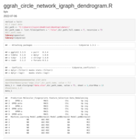
Dendrograms in R_ggplot2_cluster
cutree(hc, k = 2) # on hclust
Calculates the Gini Impurity
Gini purity, a measure of clustering specificity. Gini purity of 1.0 would be perfect clustering by lineage.

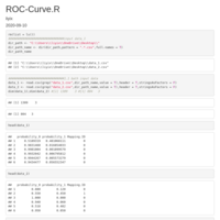
ROC-Curve
legend key backgroud
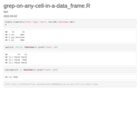
Replace the first occurrence of a character
sub function
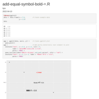
Plotting means and error bars
legend detail
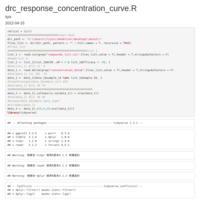
four-parameter log-logistic model
drc package
modelFit(ryegrass.m1) -----> F value
exp(e) -----> Inflection point
trim_plot
image_1 <- image_read_pdf(paste0(dir_path,dir_path_name[i]), pages = 1,density = 300)
GSEA_PLOT
Package fgsea version 1.14.0
sapply(data_5$leadingEdge, paste, collapse="/")
#####################################################
data_3$log2.fold_change <- log2(data_3$FD)
data_3$fcsign <- sign(data_3$log2.fold_change)
data_3$logP=-log10(data_3$pvalue)
data_3$metric= data_3$logP/data_3$fcsign
#############################################################